Note
Go to the end to download the full example code.
Maxwell 3D: asymmetric conductor analysis#
This example uses PyAEDT to set up the TEAM 7 problem for an asymmetric conductor with a hole and solve it using the Maxwell 3D Eddy Current solver. https://www.compumag.org/wp/wp-content/uploads/2018/06/problem7.pdf
Perform required imports#
Perform required imports.
import numpy as np
import os
import tempfile

from pyaedt import Maxwell3d
from pyaedt.generic.general_methods import write_csv
Set AEDT version#
Set AEDT version.
aedt_version = "2024.1"
Create temporary directory#
Create temporary directory.
temp_dir = tempfile.TemporaryDirectory(suffix=".ansys")
Set non-graphical mode#
Set non-graphical mode.
You can set non_graphical either to True or False.
non_graphical = False
Launch AEDT and Maxwell 3D#
Launch AEDT and Maxwell 3D. The following code sets up the project and design names, the solver, and
the version. It also creates an instance of the Maxwell3d class named m3d.
project_name = "COMPUMAG"
design_name = "TEAM 7 Asymmetric Conductor"
solver = "EddyCurrent"

m3d = Maxwell3d(
    project=project_name,
    design=design_name,
    solution_type=solver,
    version=aedt_version,
    non_graphical=non_graphical,
    new_desktop=True
)
m3d.modeler.model_units = "mm"
C:\actions-runner\_work\_tool\Python\3.10.9\x64\lib\subprocess.py:1072: ResourceWarning: subprocess 7892 is still running
  _warn("subprocess %s is still running" % self.pid,
C:\actions-runner\_work\pyaedt\pyaedt\.venv\lib\site-packages\pyaedt\generic\settings.py:428: ResourceWarning: unclosed file <_io.TextIOWrapper name='D:\\Temp\\pyaedt_ansys.log' mode='a' encoding='cp1252'>
  self._logger = val
Add Maxwell 3D setup#
Add a Maxwell 3D setup with frequency points at DC, 50 Hz, and 200Hz. Otherwise, the default PyAEDT setup values are used. To approximate a DC field in the Eddy Current solver, use a low frequency value. Second-order shape functions improve the smoothness of the induced currents in the plate.
dc_freq = 0.1
stop_freq = 50

setup = m3d.create_setup(name="Setup1")
setup.props["Frequency"] = "200Hz"
setup.props["HasSweepSetup"] = True
setup.add_eddy_current_sweep("LinearStep", dc_freq, stop_freq, stop_freq - dc_freq, clear=True)
setup.props["UseHighOrderShapeFunc"] = True
setup.props["PercentError"] = 0.4
setup.update()
True
Define coil dimensions#
Define coil dimensions as shown on the TEAM7 drawing of the coil.
coil_external = 150 + 25 + 25
coil_internal = 150
coil_r1 = 25
coil_r2 = 50
coil_thk = coil_r2 - coil_r1
coil_height = 100
coil_centre = [294 - 25 - 150 / 2, 25 + 150 / 2, 19 + 30 + 100 / 2]

# Use expressions to construct the three dimensions needed to describe the midpoints of
# the coil.

dim1 = coil_internal / 2 + (coil_external - coil_internal) / 4
dim2 = coil_internal / 2 - coil_r1
dim3 = dim2 + np.sqrt(((coil_r1 + (coil_r2 - coil_r1) / 2) ** 2) / 2)

# Use coordinates to draw a polyline along which to sweep the coil cross sections.
P1 = [dim1, -dim2, 0]
P2 = [dim1, dim2, 0]
P3 = [dim3, dim3, 0]
P4 = [dim2, dim1, 0]
Create coordinate system for positioning coil#
Create a coordinate system for positioning the coil.
m3d.modeler.create_coordinate_system(origin=coil_centre, mode="view", view="XY", name="Coil_CS")
<pyaedt.modeler.cad.Modeler.CoordinateSystem object at 0x0000018804C41840>
Create polyline#
Create a polyline. One quarter of the coil is modeled by sweeping a 2D sheet along a polyline.
<pyaedt.modeler.cad.object3d.Object3d object at 0x0000018804C40F10>
Duplicate and unite polyline to create full coil#
Duplicate and unit the polyline to create a full coil.
m3d.modeler.duplicate_around_axis(
    "Coil", axis="Global", angle=90, clones=4, create_new_objects=True, is_3d_comp=False
)
m3d.modeler.unite("Coil, Coil_1, Coil_2")
m3d.modeler.unite("Coil, Coil_3")
m3d.modeler.fit_all()
Assign material and if solution is allowed inside coil#
Assign the material Cooper from the Maxwell internal library to the coil and
allow a solution inside the coil.
m3d.assign_material("Coil", "Copper")
m3d.solve_inside("Coil")
True
Create terminal#
Create a terminal for the coil from a cross-section that is split and one half deleted.
m3d.modeler.section("Coil", "YZ")
m3d.modeler.separate_bodies("Coil_Section1")
m3d.modeler.delete("Coil_Section1_Separate1")

# Add variable for coil excitation
# ~~~~~~~~~~~~~~~~~~~~~~~~~~~~~~~~
# Add a design variable for coil excitation. The NB units here are AmpereTurns.

Coil_Excitation = 2742
m3d["Coil_Excitation"] = str(Coil_Excitation) + "A"
m3d.assign_current(assignment="Coil_Section1", amplitude="Coil_Excitation", solid=False)
m3d.modeler.set_working_coordinate_system("Global")
True
Add a material#
Add a material named team3_aluminium.
mat = m3d.materials.add_material("team7_aluminium")
mat.conductivity = 3.526e7
Model aluminium plate with a hole#
Model the aluminium plate with a hole by subtracting two rectangular cuboids.
plate = m3d.modeler.create_box(origin=[0, 0, 0], sizes=[294, 294, 19], name="Plate", material="team7_aluminium")
m3d.modeler.fit_all()
m3d.modeler.create_box(origin=[18, 18, 0], sizes=[108, 108, 19], name="Hole")
m3d.modeler.subtract(blank_list="Plate", tool_list=["Hole"], keep_originals=False)
True
Draw a background region#
Draw a background region that uses the default properties for an air region.
m3d.modeler.create_air_region(x_pos=100, y_pos=100, z_pos=100, x_neg=100, y_neg=100, z_neg=100)
<pyaedt.modeler.cad.object3d.Object3d object at 0x000001880009CA60>
Adjust eddy effects for plate and coil#
Adjust the eddy effects for the plate and coil by turning off displacement currents for all parts. The setting for eddy effect is ignored for the stranded conductor type used in the coil.
m3d.eddy_effects_on(assignment="Plate")
m3d.eddy_effects_on(assignment=["Coil", "Region", "Line_A1_B1mesh", "Line_A2_B2mesh"], enable_eddy_effects=False,
                    enable_displacement_current=False)
True
Create expression for Z component of B in Gauss#
Create an expression for the Z component of B in Gauss using the fields calculator.
Fields = m3d.ofieldsreporter
Fields.CalcStack("clear")
Fields.EnterQty("B")
Fields.CalcOp("ScalarZ")
Fields.EnterScalarFunc("Phase")
Fields.CalcOp("AtPhase")
Fields.EnterScalar(10000)
Fields.CalcOp("*")
Fields.CalcOp("Smooth")
Fields.AddNamedExpression("Bz", "Fields")
Draw two lines along which to plot Bz#
Draw two lines along which to plot Bz. The following code also adds a small cylinder to refine the mesh locally around each line.
lines = ["Line_A1_B1", "Line_A2_B2"]
mesh_diameter = "2mm"

line_points_1 = [["0mm", "72mm", "34mm"], ["288mm", "72mm", "34mm"]]
polyline = m3d.modeler.create_polyline(points=line_points_1, name=lines[0])
l1_mesh = m3d.modeler.create_polyline(points=line_points_1, name=lines[0] + "mesh")
l1_mesh.set_crosssection_properties(type="Circle", width=mesh_diameter)

line_points_2 = [["0mm", "144mm", "34mm"], ["288mm", "144mm", "34mm"]]
polyline2 = m3d.modeler.create_polyline(points=line_points_2, name=lines[1])
l2_mesh = m3d.modeler.create_polyline(points=line_points_2, name=lines[1] + "mesh")
l2_mesh.set_crosssection_properties(type="Circle", width=mesh_diameter)
<pyaedt.modeler.cad.object3d.Object3d object at 0x00000187E77E03A0>
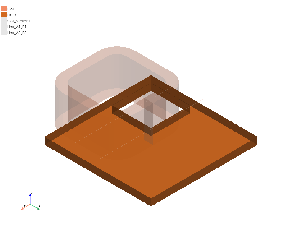
Plot model#
Plot the model.
m3d.plot(show=False, output_file=os.path.join(temp_dir.name, "model.jpg"), plot_air_objects=False)
<pyaedt.generic.plot.ModelPlotter object at 0x000001880009DC90>
Published measurement results are included with this script via the list below. Test results are used to create text files for import into a rectangular plot and to overlay simulation results.
dataset = [
    "Bz A1_B1 000 0",
    "Bz A1_B1 050 0",
    "Bz A1_B1 050 90",
    "Bz A1_B1 200 0",
    "Bz A1_B1 200 90",
    "Bz A2_B2 050 0",
    "Bz A2_B2 050 90",
    "Bz A2_B2 200 0",
    "Bz A2_B2 200 90",
]
header = ["Distance [mm]", "Bz [Tesla]"]

line_length = [0, 18, 36, 54, 72, 90, 108, 126, 144, 162, 180, 198, 216, 234, 252, 270, 288]
data = [
    [
        -6.667,
        -7.764,
        -8.707,
        -8.812,
        -5.870,
        8.713,
        50.40,
        88.47,
        100.9,
        104.0,
        104.8,
        104.9,
        104.6,
        103.1,
        97.32,
        75.19,
        29.04,
    ],
    [
        4.90,
        -17.88,
        -22.13,
        -20.19,
        -15.67,
        0.36,
        43.64,
        78.11,
        71.55,
        60.44,
        53.91,
        52.62,
        53.81,
        56.91,
        59.24,
        52.78,
        27.61,
    ],
    [-1.16, 2.84, 4.15, 4.00, 3.07, 2.31, 1.89, 4.97, 12.61, 14.15, 13.04, 12.40, 12.05, 12.27, 12.66, 9.96, 2.36],
    [
        -3.63,
        -18.46,
        -23.62,
        -21.59,
        -16.09,
        0.23,
        44.35,
        75.53,
        63.42,
        53.20,
        48.66,
        47.31,
        48.31,
        51.26,
        53.61,
        46.11,
        24.96,
    ],
    [-1.38, 1.20, 2.15, 1.63, 1.10, 0.27, -2.28, -1.40, 4.17, 3.94, 4.86, 4.09, 3.69, 4.60, 3.48, 4.10, 0.98],
    [
        -1.83,
        -8.50,
        -13.60,
        -15.21,
        -14.48,
        -5.62,
        28.77,
        60.34,
        61.84,
        56.64,
        53.40,
        52.36,
        53.93,
        56.82,
        59.48,
        52.08,
        26.56,
    ],
    [-1.63, -0.60, -0.43, 0.11, 1.26, 3.40, 6.53, 10.25, 11.83, 11.83, 11.01, 10.58, 10.80, 10.54, 10.62, 9.03, 1.79],
    [
        -0.86,
        -7.00,
        -11.58,
        -13.36,
        -13.77,
        -6.74,
        24.63,
        53.19,
        54.89,
        50.72,
        48.03,
        47.13,
        48.25,
        51.35,
        53.35,
        45.37,
        24.01,
    ],
    [-1.35, -0.71, -0.81, -0.67, 0.15, 1.39, 2.67, 3.00, 4.01, 3.80, 4.00, 3.02, 2.20, 2.78, 1.58, 1.37, 0.93],
]
Write dataset values in a CSV file#
Dataset details are used to encode test parameters in the text files.
For example, Bz A1_B1 050 0 is the Z component of flux density B.
along line A1_B1 at 50 Hz and 0 deg.
line_length.insert(0, header[0])
for i in range(len(dataset)):
    data[i].insert(0, header[1])
    ziplist = zip(line_length, data[i])
    file_path = os.path.join(temp_dir.name, str(dataset[i]) + ".csv")
    write_csv(output_file=file_path, list_data=ziplist)
Create rectangular plots and import test data into report#
Create rectangular plots, using text file encoding to control their formatting. Import test data into correct plot and overlay with simulation results. Variations for a DC plot must have different frequency and phase than the other plots.
for item in range(len(dataset)):
    if item % 2 == 0:
        t = dataset[item]
        plot_name = t[0:3] + "Along the Line" + t[2:9] + ", " + t[9:12] + "Hz"
        if t[9:12] == "000":
            variations = {
                "Distance": ["All"],
                "Freq": [str(dc_freq) + "Hz"],
                "Phase": ["0deg"],
                "Coil_Excitation": ["All"],
            }
        else:
            variations = {
                "Distance": ["All"],
                "Freq": [t[9:12] + "Hz"],
                "Phase": ["0deg", "90deg"],
                "Coil_Excitation": ["All"],
            }
        report = m3d.post.create_report(expressions=t[0:2], variations=variations, primary_sweep_variable="Distance",
                                        report_category="Fields", context="Line_" + t[3:8], plot_name=plot_name)
        file_path = os.path.join(temp_dir.name, str(dataset[i]) + ".csv")
        report.import_traces(file_path, plot_name)
Analyze project#
Analyze the project.
m3d.analyze()
True
Create plots of induced current and flux density on surface of plate#
Create two plots of the induced current (Mag_J) and the flux density (Mag_B) on the
surface of the plate.
surf_list = m3d.modeler.get_object_faces("Plate")
intrinsic_dict = {"Freq": "200Hz", "Phase": "0deg"}
m3d.post.create_fieldplot_surface(surf_list, "Mag_J", intrinsics=intrinsic_dict, plot_name="Mag_J")
m3d.post.create_fieldplot_surface(surf_list, "Mag_B", intrinsics=intrinsic_dict, plot_name="Mag_B")
m3d.post.create_fieldplot_surface(surf_list, "Mesh", intrinsics=intrinsic_dict, plot_name="Mesh")
<pyaedt.modules.solutions.FieldPlot object at 0x000001880273BA60>
Release AEDT and clean up temporary directory#
Release AEDT and remove both the project and temporary directories.
m3d.release_desktop(True, True)
temp_dir.cleanup()
Total running time of the script: (5 minutes 21.413 seconds)