Postprocessing

Postprocessing is essential in simulation. PyAEDT offers the capability to read solutions and visualize results both within AEDT and externally using the pyvista and matplotlib packages.

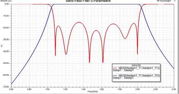
To use PyAEDT to create a report in AEDT, you can follow this general structure:

from pyaedt import Hfss
hfss = Hfss()
hfss.analyze_nominal()
hfss.post.create_report(["db(S11)", "db(S12)"])

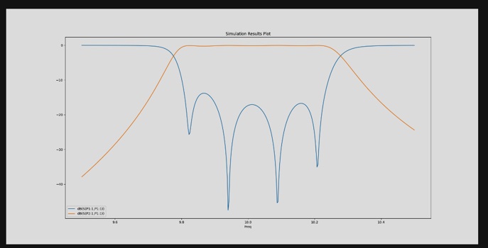
You can also generate reports in Matplotlib:

from pyaedt import Hfss
hfss = Hfss()
hfss.analyze_nominal()

traces_to_plot = hfss.get_traces_for_plot(second_element_filter="P1*")
report = hfss.post.create_report(traces_to_plot)  # Creates a report in HFSS
solution = report.get_solution_data()
plt = solution.plot(solution.expressions)  # Matplotlib axes object.

You can use PyAEDT to plot any kind of report available in the Electronics Desktop interface. To access all available category, use the reports_by_category class.

from pyaedt import Hfss
hfss = Hfss()
hfss.analyze_nominal()
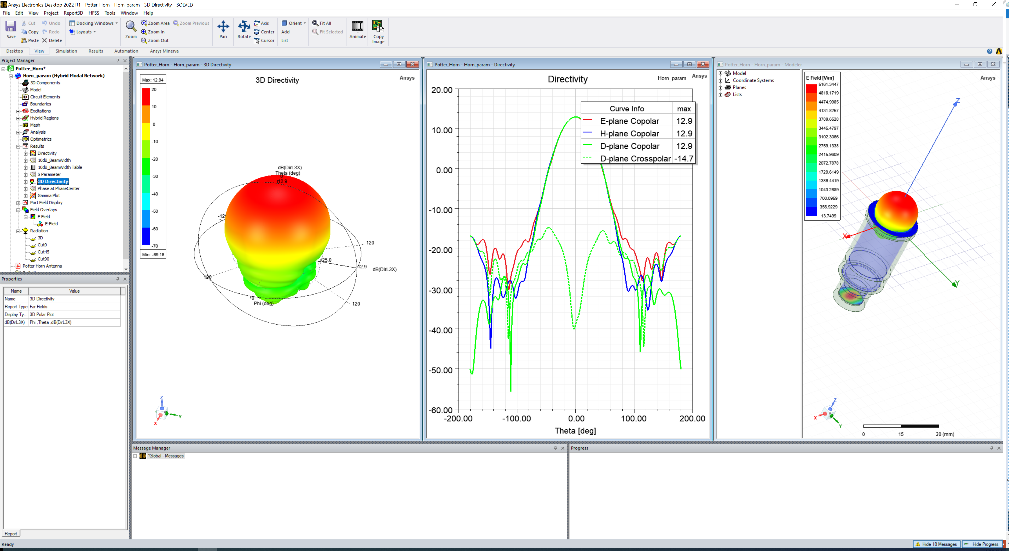
# Create a 3D far field
new_report = hfss.post.reports_by_category.far_field(expressions="db(RealizedGainTotal)",
                                                     setup=hfss.nominal_adaptive)

You can plot the field plot directly in HFSS and export it to image files.

from pyaedt import Hfss
hfss = Hfss()
hfss.analyze_nominal()

cutlist = ["Global:XY"]
setup_name = hfss.existing_analysis_sweeps[0]
quantity_name = "ComplexMag_E"
intrinsic = {"Freq": "5GHz", "Phase": "180deg"}
# Create a field plot
plot1 = hfss.post.create_fieldplot_cutplane(objlist=cutlist,
                                            quantityName=quantity_name,
                                            setup=setup_name,
                                            intrinsics=intrinsic)

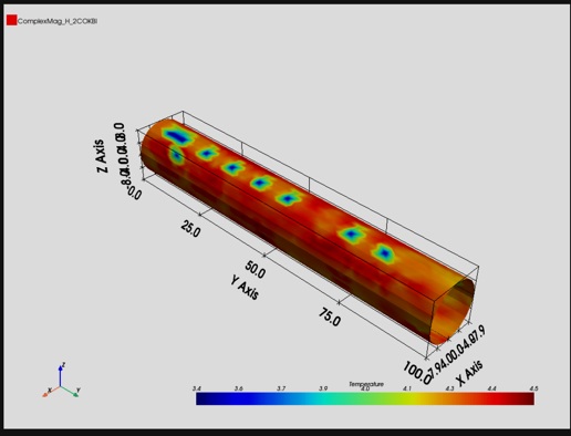
PyAEDT leverages PyVista to export and plot fields outside AEDT, generating images and animations:

from pyaedt import Hfss
hfss = Hfss()
hfss.analyze_nominal()
cutlist = ["Global:XY"]
setup_name = hfss.existing_analysis_sweeps[0]
quantity_name = "ComplexMag_E"
intrinsic = {"Freq": "5GHz", "Phase": "180deg"}
hfss.logger.info("Generating the image")
plot_obj = hfss.post.plot_field(
        quantity="Mag_E",
        objects_list=cutlist,
        plot_type="CutPlane",
        setup=setup_name,
        intrinsics=intrinsic
    )

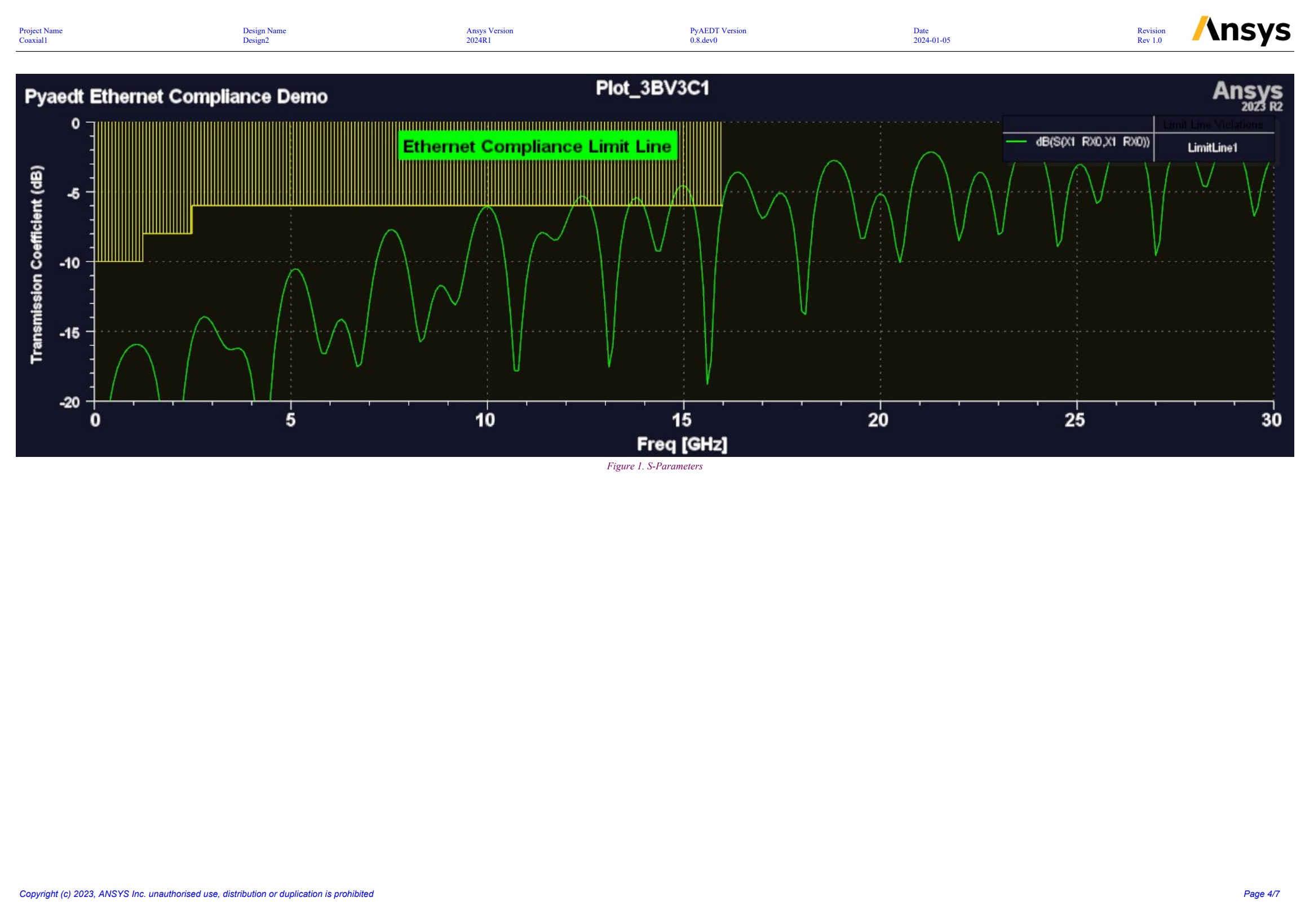
PyAEDT includes a powerful class to generate a PDF report that is based on the Python fpdf2 package.

To see the capabilities offered by PyAEDT, download a sample PDF report that uses this class:

PDF report example

This code creates the previous PDF report:

from pyaedt.generic.pdf import AnsysReport
import os
report = AnsysReport()
report.aedt_version = "2024R1"
report.template_name = "AnsysTemplate"
report.project_name = "Coaxial1"
report.design_name = "Design2"
report.template_data.font = "times"
report.create()
report.add_chapter("Chapter 1")
report.add_sub_chapter("C1")
report.add_text("Hello World.\nlorem ipsum....")
report.add_text("ciao2", True, True)
report.add_empty_line(2)
report.add_page_break()
report.add_chapter("Chapter 2")
report.add_sub_chapter("Charts")
local_path = r'C:\result'
report.add_section(portrait=False, page_format="a3")
report.add_image(os.path.join(local_path, "return_loss.jpg"), width=400, caption="S-Parameters")
report.add_section(portrait=False, page_format="a5")
report.add_table("MyTable", [["x", "y"], ["0", "1"], ["2", "3"], ["10", "20"]])
report.add_section()
report.add_chart([0, 1, 2, 3, 4, 5], [10, 20, 4, 30, 40, 12], "Freq", "Val", "MyTable")
report.add_toc()
report.save_pdf(r'c:\temp', "report_example.pdf")