Maxwell 3D: bath plate analysis

This example uses PyAEDT to set up the TEAM 3 bath plate problem and solve it using the Maxwell 3D Eddy Current solver.

Perform required imports

Perform required imports.

import os
import pyaedt

Set non-graphical mode

Set non-graphical mode. You can set non_graphical either to True or False.

non_graphical = False

Launch AEDT and Maxwell 3D

Launch AEDT and Maxwell 3D after first setting up the project and design names, the solver, and the version. The following code also creates an instance of the Maxwell3d class named M3D.

project_name = "COMPUMAG"
design_name = "TEAM 3 Bath Plate"
Solver = "EddyCurrent"
desktop_version = "2023.2"

m3d = pyaedt.Maxwell3d(
    projectname=pyaedt.generate_unique_project_name(),
    designname=design_name,
    solution_type=Solver,
    specified_version=desktop_version,
    non_graphical=non_graphical,
    new_desktop_session=True,
)
uom = m3d.modeler.model_units = "mm"
modeler = m3d.modeler

Initializing new desktop!

Add variable

Add a design variable named Coil_Position that you use later to adjust the position of the coil.

Coil_Position = -20
m3d["Coil_Position"] = str(Coil_Position) + uom  # Creates a design variable in Maxwell

Add material

Add a material named team3_aluminium for the ladder plate.

mat = m3d.materials.add_material("team3_aluminium")
mat.conductivity = 32780000

Draw background region

Draw a background region that uses the default properties for an air region.

m3d.modeler.create_air_region(x_pos=100, y_pos=100, z_pos=100, x_neg=100, y_neg=100, z_neg=100)

<pyaedt.modeler.cad.object3d.Object3d object at 0x000001D9CCD43370>

Draw ladder plate and assign material

Draw a ladder plate and assign it the newly created material team3_aluminium.

m3d.modeler.create_box(position=[-30, -55, 0], dimensions_list=[60, 110, -6.35], name="LadderPlate",
                       matname="team3_aluminium")
m3d.modeler.create_box(position=[-20, -35, 0], dimensions_list=[40, 30, -6.35], name="CutoutTool1")
m3d.modeler.create_box(position=[-20, 5, 0], dimensions_list=[40, 30, -6.35], name="CutoutTool2")
m3d.modeler.subtract("LadderPlate", ["CutoutTool1", "CutoutTool2"], keep_originals=False)

True

Add mesh refinement to ladder plate

Add a mesh refinement to the ladder plate.

m3d.mesh.assign_length_mesh("LadderPlate", maxlength=3, maxel=None, meshop_name="Ladder_Mesh")

<pyaedt.modules.Mesh.MeshOperation object at 0x000001D9CCD436A0>

Draw search coil and assign excitation

Draw a search coil and assign it a stranded current excitation. The stranded type forces the current density to be constant in the coil.

m3d.modeler.create_cylinder(
    cs_axis="Z", position=[0, "Coil_Position", 15], radius=40, height=20, name="SearchCoil", matname="copper"
)
m3d.modeler.create_cylinder(
    cs_axis="Z", position=[0, "Coil_Position", 15], radius=20, height=20, name="Bore", matname="copper"
)
m3d.modeler.subtract("SearchCoil", "Bore", keep_originals=False)
m3d.modeler.section("SearchCoil", "YZ")
m3d.modeler.separate_bodies("SearchCoil_Section1")
m3d.modeler.delete("SearchCoil_Section1_Separate1")
m3d.assign_current(object_list=["SearchCoil_Section1"], amplitude=1260, solid=False, name="SearchCoil_Excitation")

<pyaedt.modules.Boundary.BoundaryObject object at 0x000001D9A4252C50>

Draw a line for plotting Bz

Draw a line for plotting Bz later. Bz is the Z component of the flux density. The following code also adds a small diameter cylinder to refine the mesh locally around the line.

Line_Points = [["0mm", "-55mm", "0.5mm"], ["0mm", "55mm", "0.5mm"]]
P1 = modeler.create_polyline(position_list=Line_Points, name="Line_AB")
P2 = modeler.create_polyline(position_list=Line_Points, name="Line_AB_MeshRefinement")
P2.set_crosssection_properties(type="Circle", width="0.5mm")

<pyaedt.modeler.cad.polylines.Polyline object at 0x000001D9A4253160>

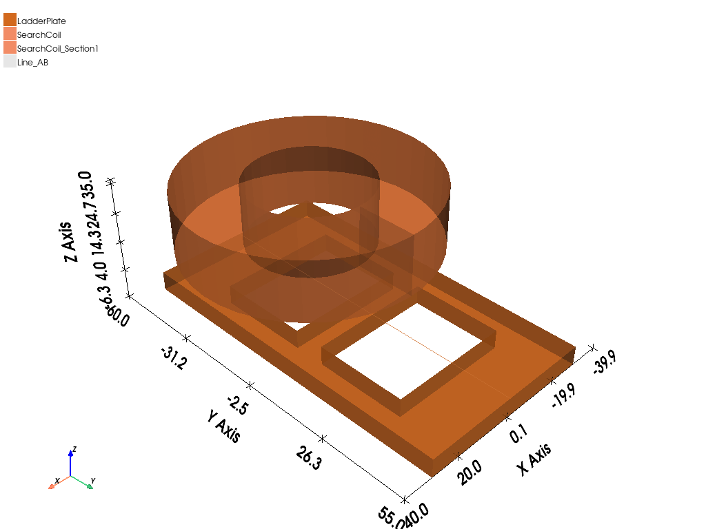
Plot model

Plot the model.

m3d.plot(show=False, export_path=os.path.join(m3d.working_directory, "Image.jpg"), plot_air_objects=False)

<pyaedt.generic.plot.ModelPlotter object at 0x000001D9A4250B80>

Add Maxwell 3D setup

Add a Maxwell 3D setup with frequency points at 50 Hz and 200 Hz.

Setup = m3d.create_setup(setupname="Setup1")
Setup.props["Frequency"] = "200Hz"
Setup.props["HasSweepSetup"] = True
Setup.add_eddy_current_sweep(range_type="LinearStep", start=50, end=200, count=150, clear=True)

True

Adjust eddy effects

Adjust eddy effects for the ladder plate and the search coil. The setting for eddy effect is ignored for the stranded conductor type used in the search coil.

m3d.eddy_effects_on(["LadderPlate"], activate_eddy_effects=True, activate_displacement_current=True)
m3d.eddy_effects_on(["SearchCoil"], activate_eddy_effects=False, activate_displacement_current=True)

True

Add linear parametric sweep

Add a linear parametric sweep for the two coil positions.

sweepname = "CoilSweep"
param = m3d.parametrics.add("Coil_Position", -20, 0, 20, "LinearStep", parametricname=sweepname)
param["SaveFields"] = True
param["CopyMesh"] = False
param["SolveWithCopiedMeshOnly"] = True

# Solve parametric sweep
# ~~~~~~~~~~~~~~~~~~~~~~
# Solve the parametric sweep directly so that results of all variations are available.

m3d.analyze_setup(sweepname)

True

Create expression for Bz

Create an expression for Bz using the fields calculator.

Fields = m3d.odesign.GetModule("FieldsReporter")
Fields.EnterQty("B")
Fields.CalcOp("ScalarZ")
Fields.EnterScalar(1000)
Fields.CalcOp("*")
Fields.CalcOp("Smooth")
Fields.AddNamedExpression("Bz", "Fields")

Plot mag(Bz) as a function of frequency

Plot mag(Bz) as a function of frequency for both coil positions.

variations = {"Distance": ["All"], "Freq": ["All"], "Phase": ["0deg"], "Coil_Position": ["-20mm"]}
m3d.post.create_report(
    expressions="mag(Bz)",
    report_category="Fields",
    context="Line_AB",
    variations=variations,
    primary_sweep_variable="Distance",
    plotname="mag(Bz) Along 'Line_AB' Offset Coil",
)

variations = {"Distance": ["All"], "Freq": ["All"], "Phase": ["0deg"], "Coil_Position": ["0mm"]}
m3d.post.create_report(
    expressions="mag(Bz)",
    report_category="Fields",
    context="Line_AB",
    variations=variations,
    primary_sweep_variable="Distance",
    plotname="mag(Bz) Along 'Line_AB' Coil",
)

<pyaedt.modules.report_templates.Fields object at 0x000001D9A4253400>

Generate plot outside of AEDT

Generate the same plot outside AEDT.

variations = {"Distance": ["All"], "Freq": ["All"], "Phase": ["0deg"], "Coil_Position": ["All"]}

solutions = m3d.post.get_solution_data(
    expressions="mag(Bz)",
    report_category="Fields",
    context="Line_AB",
    variations=variations,
    primary_sweep_variable="Distance",
)

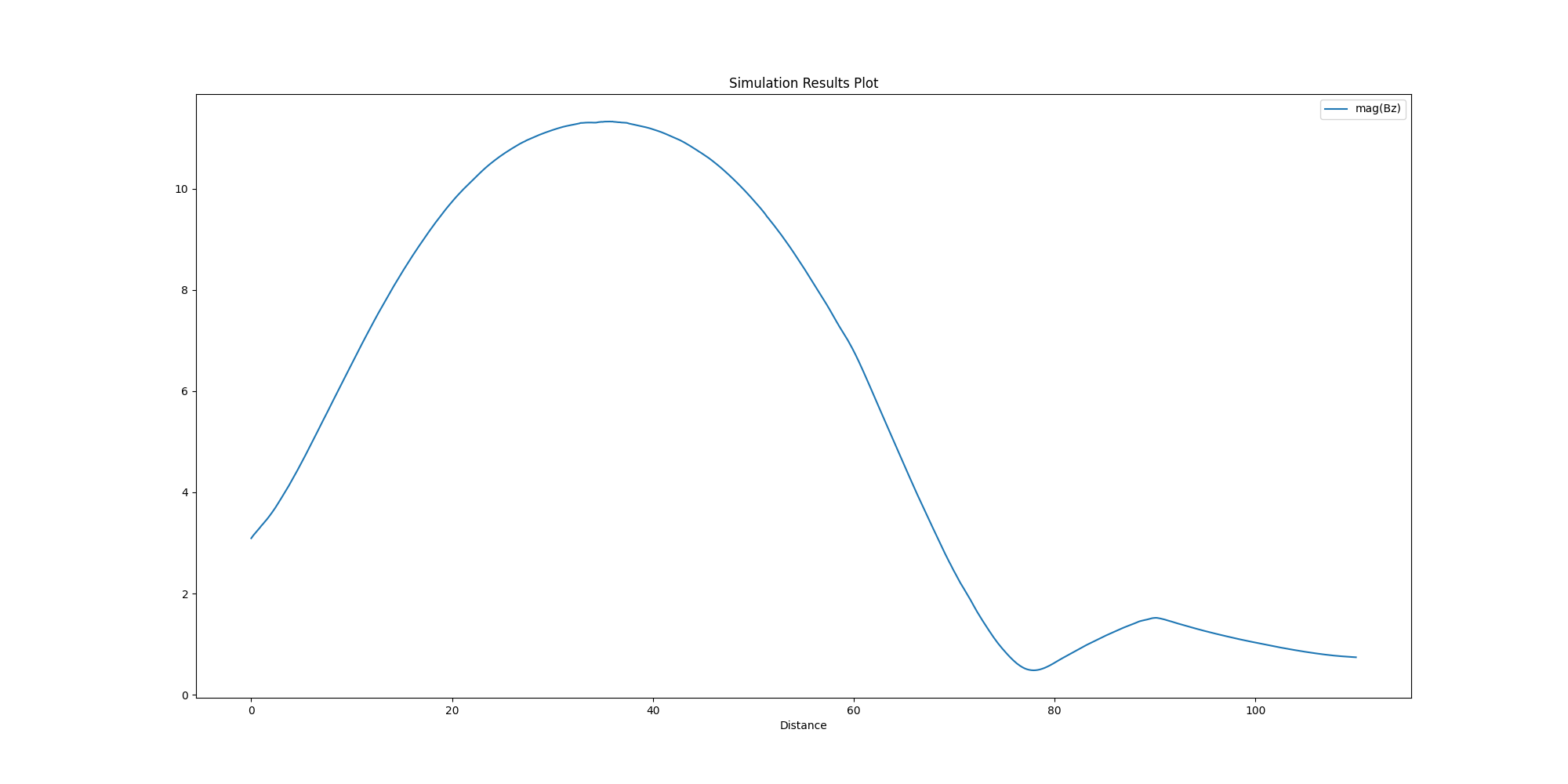
Set up sweep value and plot solution

Set up a sweep value and plot the solution.

solutions.active_variation["Coil_Position"] = -0.02
solutions.plot()

<Figure size 2000x1000 with 1 Axes>

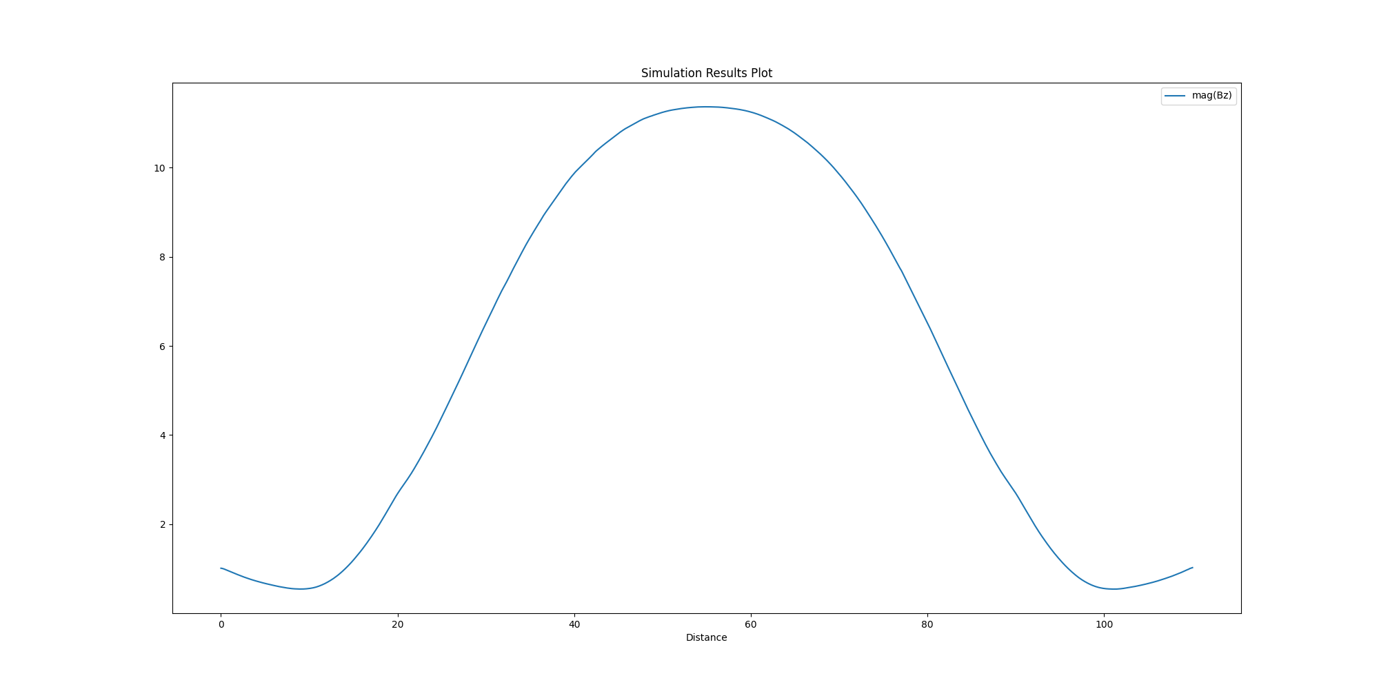
Change sweep value and plot solution

Change the sweep value and plot the solution again.

solutions.active_variation["Coil_Position"] = 0
solutions.plot()

<Figure size 2000x1000 with 1 Axes>

Plot induced current density on surface of ladder plate

Plot the induced current density, "Mag_J", on the surface of the ladder plate.

surflist = modeler.get_object_faces("LadderPlate")
intrinsic_dict = {"Freq": "50Hz", "Phase": "0deg"}
m3d.post.create_fieldplot_surface(surflist, "Mag_J", intrinsincDict=intrinsic_dict, plot_name="Mag_J")

<pyaedt.modules.solutions.FieldPlot object at 0x000001D9A65AECB0>

Release AEDT

Release AEDT from the script engine, leaving both AEDT and the project open.

m3d.release_desktop(True, True)

True