Note
Go to the end to download the full example code.
HFSS: dipole antenna#
This example shows how you can use PyAEDT to create a dipole antenna in HFSS and postprocess results.
Perform required imports#
Perform required imports.
import os
import pyaedt

project_name = pyaedt.generate_unique_project_name(project_name="dipole")
Set AEDT version#
Set AEDT version.
aedt_version = "2024.1"
Set non-graphical mode#
Set non-graphical mode. `
You can set non_graphical either to True or False.
non_graphical = False
Launch AEDT#
Launch AEDT 2023 R2 in graphical mode.
d = pyaedt.launch_desktop(aedt_version, non_graphical=non_graphical, new_desktop=True)
Launch HFSS#
Launch HFSS 2023 R2 in graphical mode.
hfss = pyaedt.Hfss(project=project_name, solution_type="Modal")
Define variable#
Define a variable for the dipole length.
hfss["l_dipole"] = "13.5cm"
Get 3D component from system library#
Get a 3D component from the syslib directory. For this example to run
correctly, you must get all geometry parameters of the 3D component or, in
case of an encrypted 3D component, create a dictionary of the parameters.
compfile = hfss.components3d["Dipole_Antenna_DM"]
geometryparams = hfss.get_components3d_vars("Dipole_Antenna_DM")
geometryparams["dipole_length"] = "l_dipole"
hfss.modeler.insert_3d_component(compfile, geometryparams)
<pyaedt.modeler.cad.components_3d.UserDefinedComponent object at 0x00000187CB5580D0>
Create boundaries#
Create boundaries. A region with openings is needed to run the analysis.
hfss.create_open_region(frequency="1GHz")
True
Plot model#
Plot the model.
my_plot = hfss.plot(show=False, plot_air_objects=False)
my_plot.show_axes = False
my_plot.show_grid = False
my_plot.isometric_view = False
my_plot.plot(
    os.path.join(hfss.working_directory, "Image.jpg"),
)

True
Create setup#
Create a setup with a sweep to run the simulation.
setup = hfss.create_setup("MySetup")
setup.props["Frequency"] = "1GHz"
setup.props["MaximumPasses"] = 1
hfss.create_linear_count_sweep(setup=setup.name, units="GHz", start_frequency=0.5, stop_frequency=1.5,
                               num_of_freq_points=251, name="sweep1", save_fields=False, sweep_type="Interpolating",
                               interpolation_tol=3, interpolation_max_solutions=255)
<pyaedt.modules.SolveSweeps.SweepHFSS object at 0x00000187CB55B040>
Save and run simulation#
Save and run the simulation.
hfss.analyze_setup("MySetup")
True
Create scattering plot and far fields report#
Create a scattering plot and a far fields report.
hfss.create_scattering("MyScattering")
variations = hfss.available_variations.nominal_w_values_dict
variations["Freq"] = ["1GHz"]
variations["Theta"] = ["All"]
variations["Phi"] = ["All"]
hfss.post.create_report("db(GainTotal)", hfss.nominal_adaptive, variations, primary_sweep_variable="Theta",
                        report_category="Far Fields", context="3D")
<pyaedt.modules.report_templates.FarField object at 0x00000187CB558B50>
Create far fields report using report objects#
Create a far fields report using the report_by_category.far field method,
which gives you more freedom.
new_report = hfss.post.reports_by_category.far_field("db(RealizedGainTotal)", hfss.nominal_adaptive, "3D")
new_report.variations = variations
new_report.primary_sweep = "Theta"
new_report.create("Realized2D")
True
Generate multiple plots#
Generate multiple plots using the object new_report. This code generates
2D and 3D polar plots.
new_report.report_type = "3D Polar Plot"
new_report.secondary_sweep = "Phi"
new_report.create("Realized3D")
True
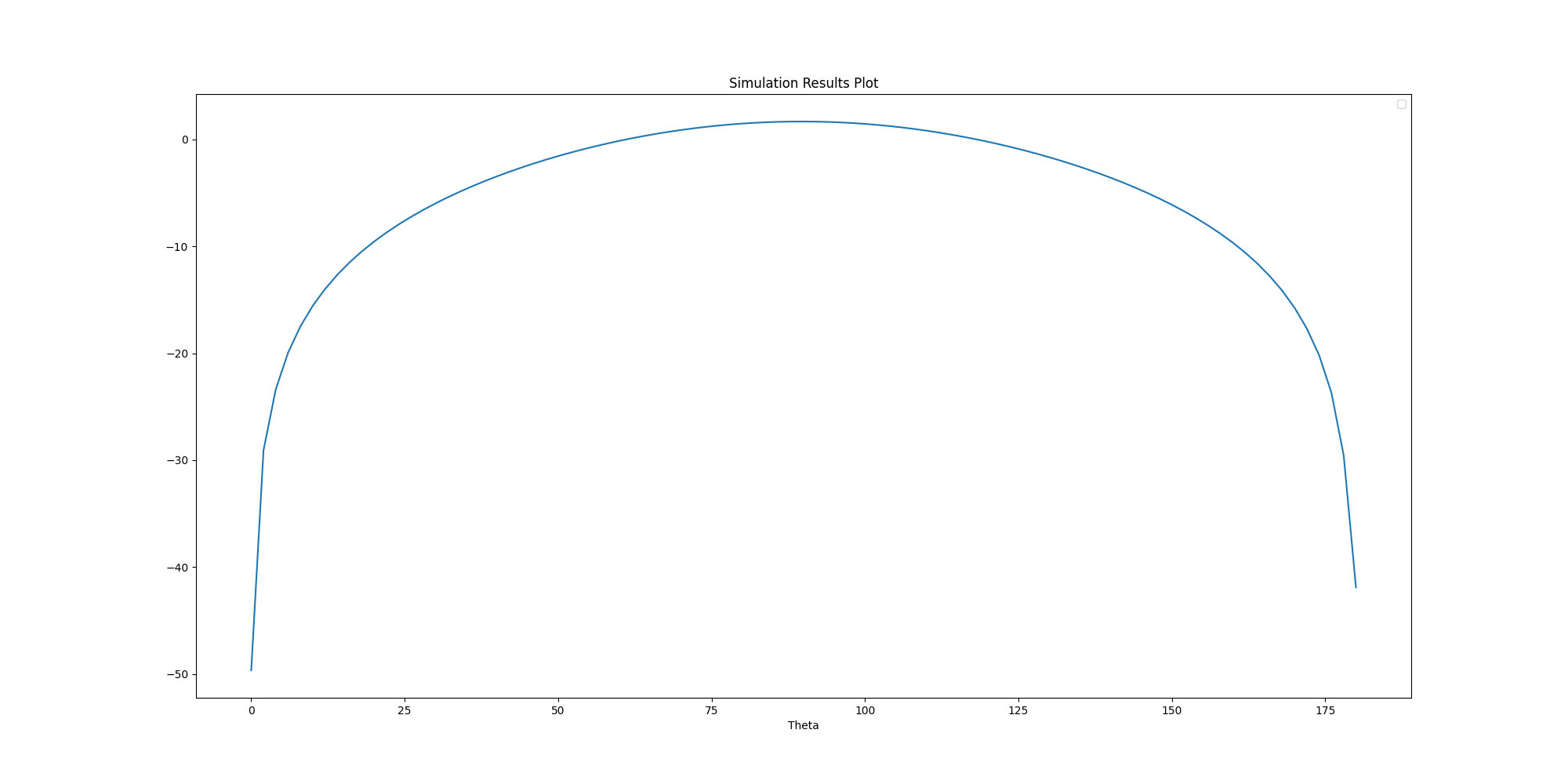
Get solution data#
Get solution data using the object new_report` and postprocess or plot the
data outside AEDT.
solution_data = new_report.get_solution_data()
solution_data.plot()
<Figure size 2000x1000 with 1 Axes>
Generate far field plot#
Generate a far field plot by creating a postprocessing variable and assigning
it to a new coordinate system. You can use the post prefix to create a
postprocessing variable directly from a setter, or you can use the set_variable
method with an arbitrary name.
hfss["post_x"] = 2
hfss.variable_manager.set_variable(name="y_post", expression=1, is_post_processing=True)
hfss.modeler.create_coordinate_system(origin=["post_x", "y_post", 0], name="CS_Post")
hfss.insert_infinite_sphere(custom_coordinate_system="CS_Post", name="Sphere_Custom")
<pyaedt.modules.Boundary.FarFieldSetup object at 0x00000187CD456530>
Get solution data#
Get solution data. You can use this code to generate the same plot outside AEDT.
new_report = hfss.post.reports_by_category.far_field("GainTotal", hfss.nominal_adaptive, "3D")
new_report.primary_sweep = "Theta"
new_report.far_field_sphere = "3D"
solutions = new_report.get_solution_data()
Generate 3D plot using Matplotlib#
Generate a 3D plot using Matplotlib.
solutions.plot_3d()
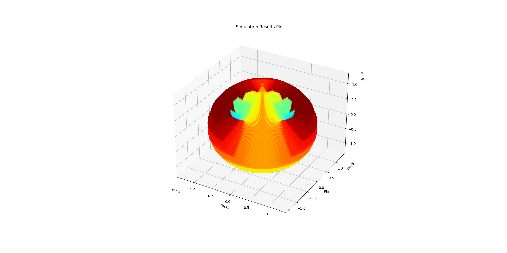
<Figure size 2000x1000 with 1 Axes>
Generate 3D far fields plot using Matplotlib#
Generate a far fields plot using Matplotlib.
new_report.far_field_sphere = "Sphere_Custom"
solutions_custom = new_report.get_solution_data()
solutions_custom.plot_3d()
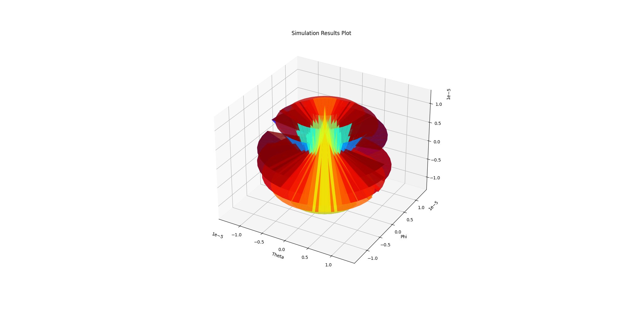
<Figure size 2000x1000 with 1 Axes>
Generate 2D plot using Matplotlib#
Generate a 2D plot using Matplotlib where you specify whether it is a polar plot or a rectangular plot.
solutions.plot()
<Figure size 2000x1000 with 1 Axes>
Get far field data#
Get far field data. After the simulation completes, the far field data is generated port by port and stored in a data class, , user can use this data once AEDT is released.
ffdata = hfss.get_antenna_ffd_solution_data(frequencies=["1000MHz"], setup=hfss.nominal_adaptive,
                                            sphere="Sphere_Custom")

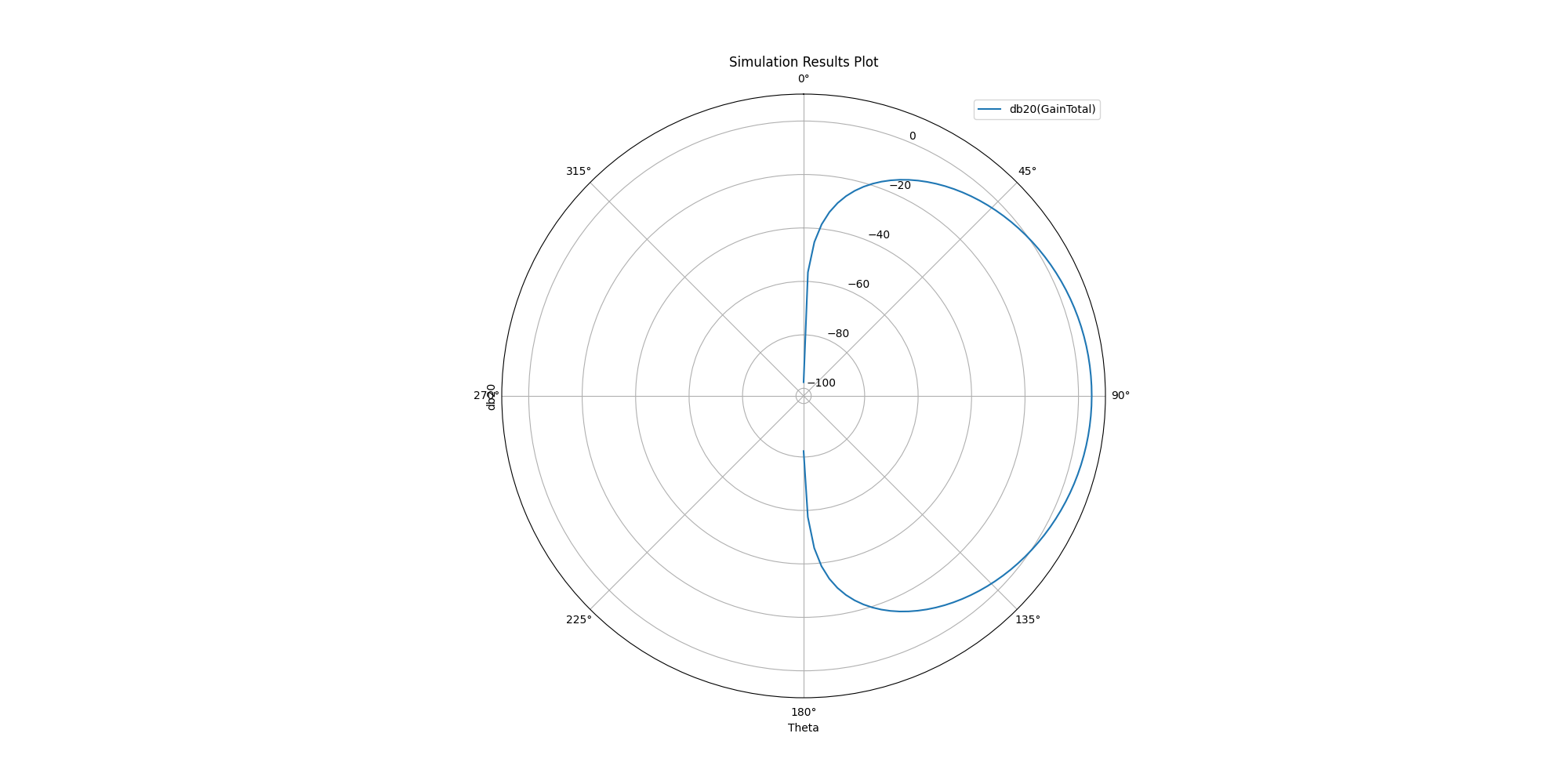
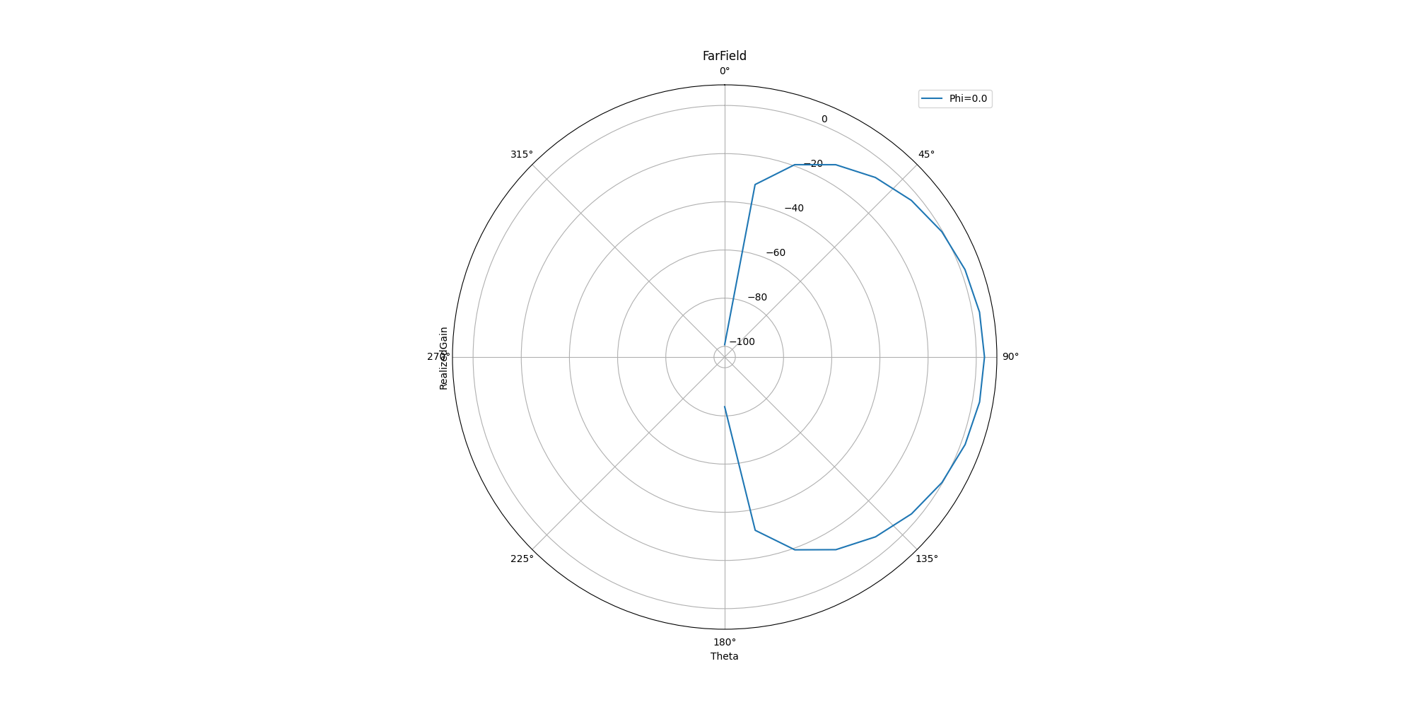
Generate 2D cutout plot#
Generate 2D cutout plot. You can define the Theta scan and Phi scan.
ffdata.plot_2d_cut(quantity='RealizedGain', primary_sweep="theta", secondary_sweep_value=0, title='FarField',
                   quantity_format="dB20", is_polar=True)
<Figure size 2000x1000 with 1 Axes>
Close AEDT#
After the simulation completes, you can close AEDT or release it using the
pyaedt.Desktop.release_desktop() method.
All methods provide for saving the project before closing.
d.release_desktop()
True
Total running time of the script: (1 minutes 7.248 seconds)