HFSS: component antenna array

This example shows how you can use PyAEDT to create an example using a 3D component file. It sets up the analysis, solves it, and uses postprocessing functions to create plots using Matplotlib and PyVista without opening the HFSS user interface. This examples runs only on Windows using CPython.

Perform required imports

Perform required imports.

import os
import pyaedt

Set non-graphical mode

Set non-graphical mode. You can set non_graphical either to True or False.

non_graphical = False

Download 3D component

Download the 3D component that is needed to run the example.

example_path = pyaedt.downloads.download_3dcomponent()

Launch HFSS and save project

Launch HFSS and save the project.

project_name = pyaedt.generate_unique_project_name(project_name="array")
hfss = pyaedt.Hfss(projectname=project_name,
                   specified_version="2023.2",
                   designname="Array_Simple",
                   non_graphical=non_graphical,
                   new_desktop_session=True)

print("Project name " + project_name)

Initializing new desktop!
Project name D:\Temp\pyaedt_prj_CH4\array.aedt

Read array definition from JSON file

Read the array definition from a JSON file. A JSON file can contain all information needed to import and set up a full array in HFSS.

If a 3D component is not available in the design, it is loaded into the dictionary from the path that you specify. The following code edits the dictionary to point to the location of the A3DCOMP file.

dict_in = pyaedt.data_handler.json_to_dict(os.path.join(example_path, "array_simple.json"))
dict_in["Circ_Patch_5GHz1"] = os.path.join(example_path, "Circ_Patch_5GHz.a3dcomp")
dict_in["cells"][(3, 3)] = {"name": "Circ_Patch_5GHz1"}
hfss.add_3d_component_array_from_json(dict_in)

True

Set up simulation

Set up a simulation and analyze it.

setup = hfss.create_setup()
setup.props["Frequency"] = "5GHz"
setup.props["MaximumPasses"] = 3

hfss.analyze(num_cores=4)

True

Get far field data

Get far field data. After the simulation completes, the far field data is generated port by port and stored in a data class.

ffdata = hfss.get_antenna_ffd_solution_data(sphere_name="Infinite Sphere1", setup_name=hfss.nominal_adaptive,
                                            frequencies=[5e9])

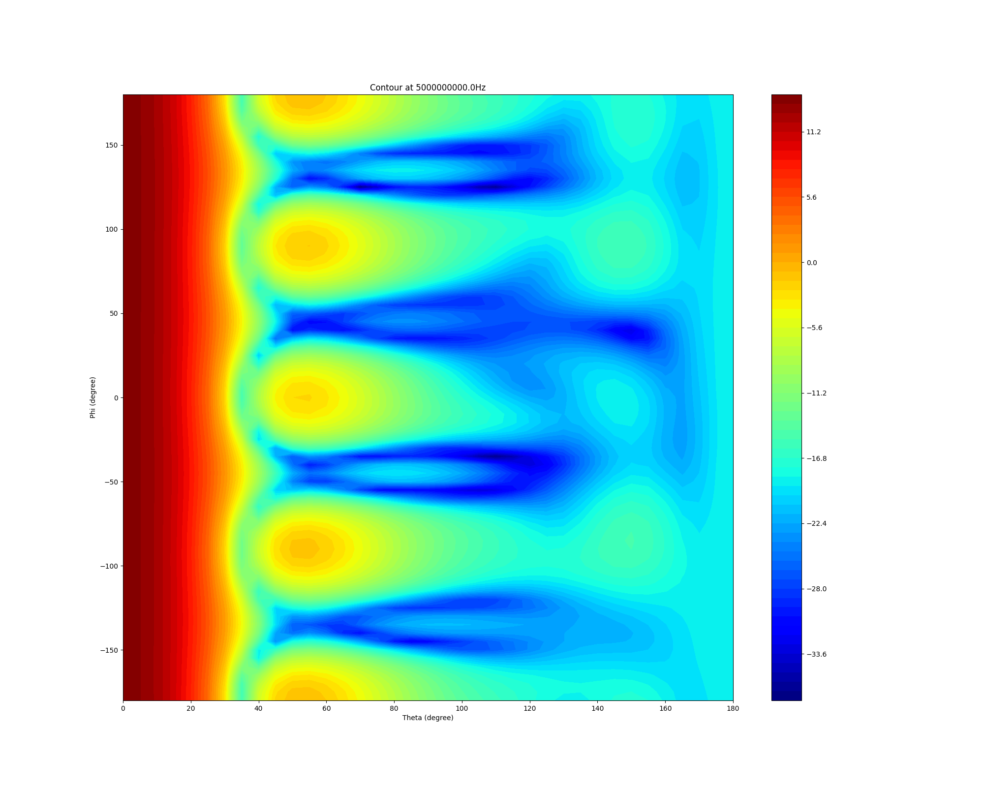
Generate contour plot

Generate a contour plot. You can define the Theta scan and Phi scan.

ffdata.plot_farfield_contour(qty_str='RealizedGain', convert_to_db=True,
                             title='Contour at {}Hz'.format(ffdata.frequency))

<module 'matplotlib.pyplot' from 'C:\\actions-runner\\_work\\pyaedt\\pyaedt\\testenv\\lib\\site-packages\\matplotlib\\pyplot.py'>

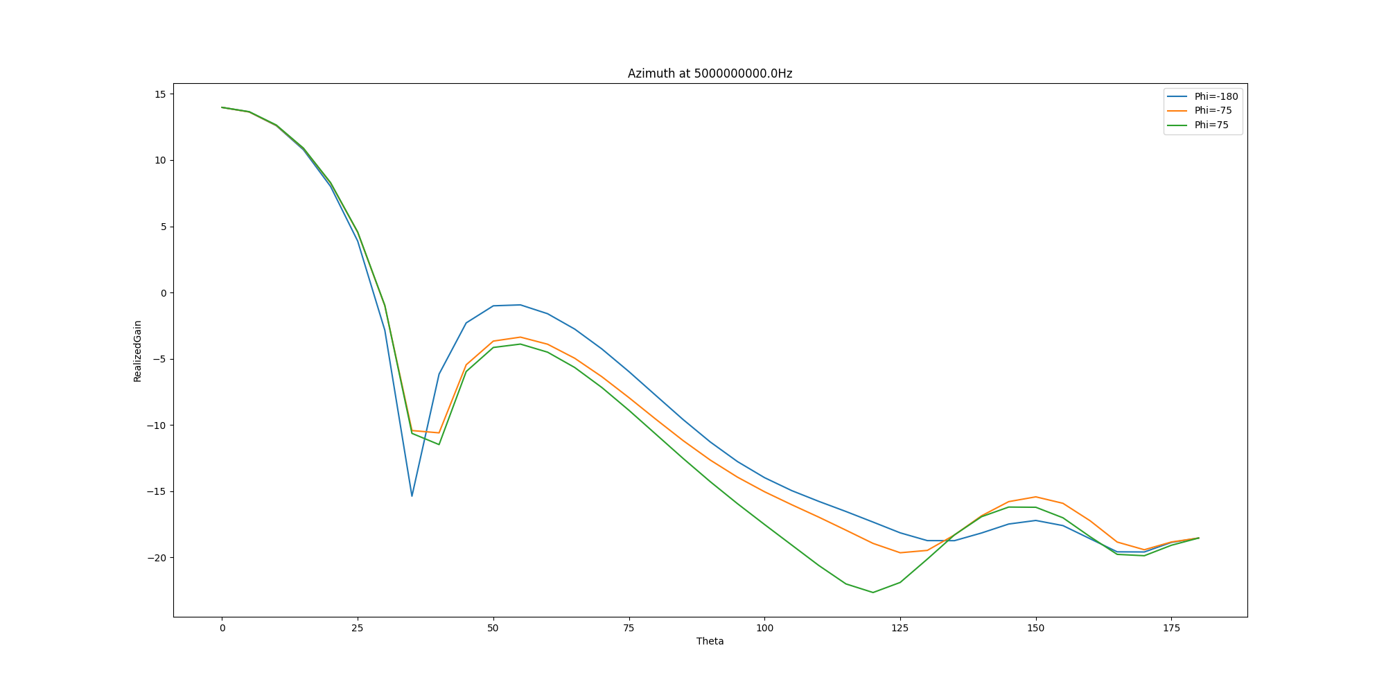
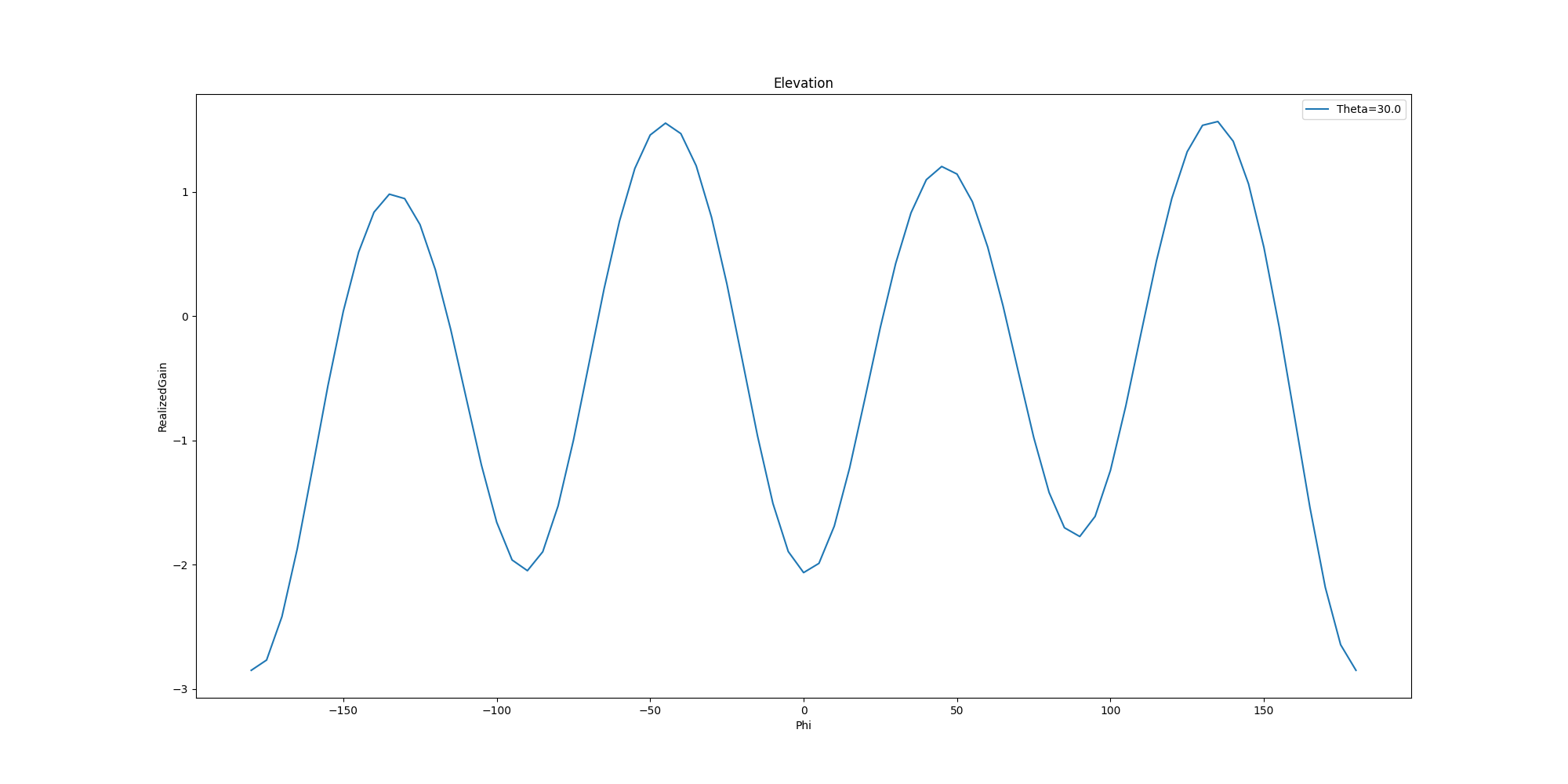
Generate 2D cutout plots

Generate 2D cutout plots. You can define the Theta scan and Phi scan.

ffdata.plot_2d_cut(primary_sweep='theta', secondary_sweep_value=[-180, -75, 75],
                   qty_str='RealizedGain',
                   title='Azimuth at {}Hz'.format(ffdata.frequency),
                   convert_to_db=True)

ffdata.plot_2d_cut(primary_sweep="phi", secondary_sweep_value=30,
                   qty_str='RealizedGain',
                   title='Elevation',
                   convert_to_db=True)

• 
• 

<Figure size 2000x1000 with 1 Axes>

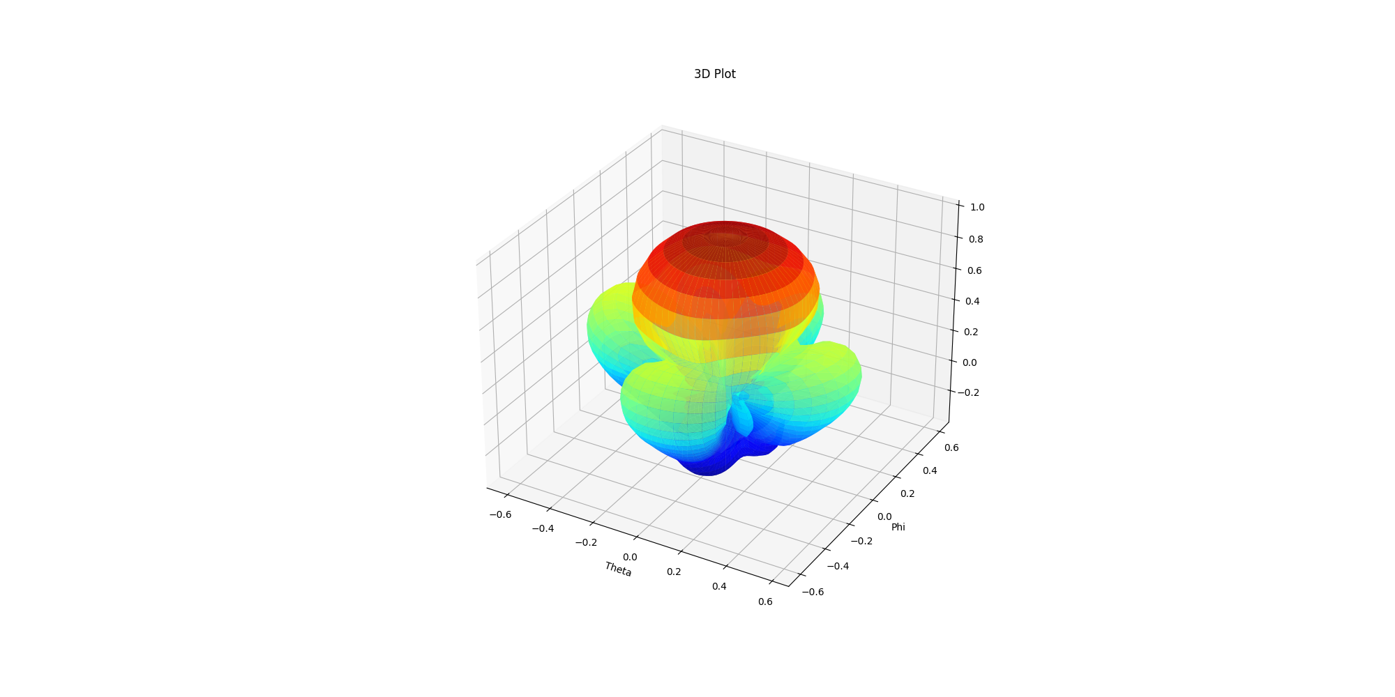
Generate 3D polar plots in Matplotlib

Generate 3D polar plots in Matplotlib. You can define the Theta scan and Phi scan.

ffdata.polar_plot_3d(qty_str='RealizedGain',
                     convert_to_db=True)

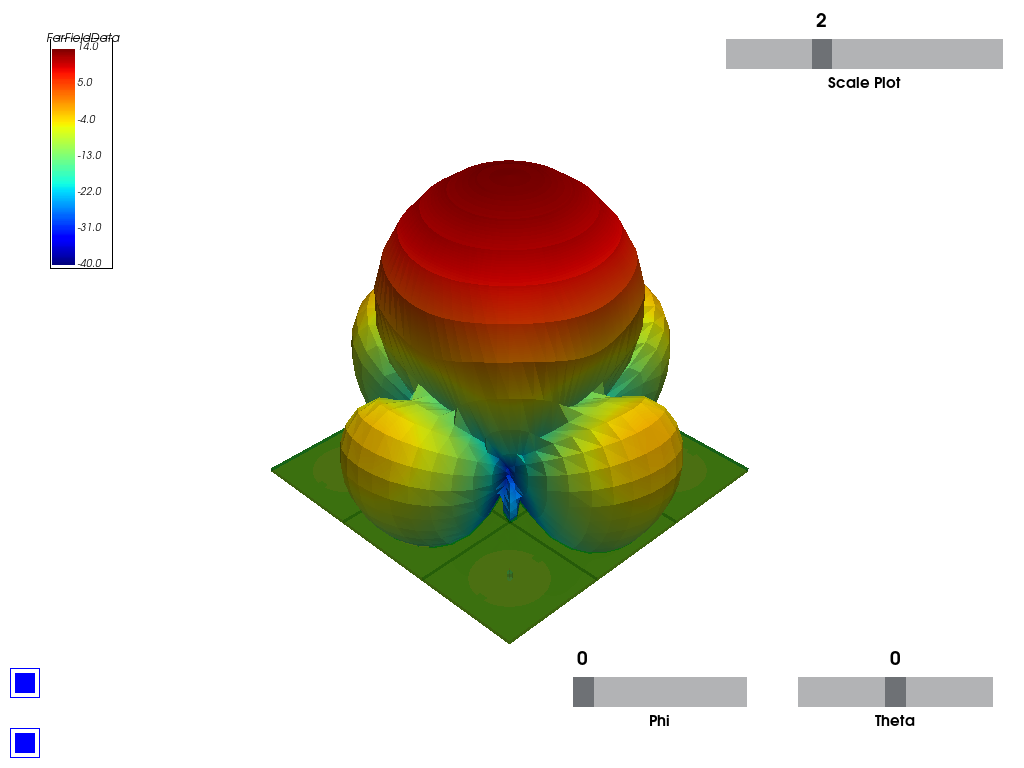
Generate 3D plots in PyVista

Generate 3D plots in PyVista. You can define the Theta and Phi scan angles. You can change the easy-to-use interactive plot that is generated on the fly.

ffdata.polar_plot_3d_pyvista(qty_str='RealizedGain',
                             convert_to_db=True,
                             export_image_path=os.path.join(hfss.working_directory, "picture.jpg"),
                             show=False)

• 
• 

C:\actions-runner\_work\pyaedt\pyaedt\testenv\lib\site-packages\pyvista\core\dataset.py:2123: PyVistaDeprecationWarning: Use of `DataSet.overwrite` is deprecated. Use `DataSet.copy_from` instead.
  warnings.warn(

True

Release AEDT

Release AEDT.

hfss.release_desktop()

True