Circuit: AMI PostProcessing

This example shows how you can use PyAEDT to perform advanced postprocessing of AMI simulations.

Perform required imports

Perform required imports and set the local path to the path for PyAEDT.

# sphinx_gallery_thumbnail_path = 'Resources/spectrum_plot.png'

import os
from matplotlib import pyplot as plt
import numpy as np

import pyaedt

# Set local path to path for PyAEDT
temp_folder = pyaedt.generate_unique_folder_name()
project_path = pyaedt.downloads.download_file("ami", "ami_usb.aedtz", temp_folder)

Set AEDT version

Set AEDT version.

aedt_version = "2024.1"

Set non-graphical mode

Set non-graphical mode. You can set non_graphical either to True or False. The Boolean parameter new_thread defines whether to create a new instance of AEDT or try to connect to an existing instance of it.

non_graphical = False
NewThread = True

Launch AEDT with Circuit and enable Pandas as the output format

All outputs obtained with the get_solution_data method will have the Pandas format. Launch AEDT with Circuit. The pyaedt.Desktop class initializes AEDT and starts the specified version in the specified mode.

pyaedt.settings.enable_pandas_output = True
cir = pyaedt.Circuit(projectname=os.path.join(project_path), non_graphical=non_graphical,
                     specified_version=aedt_version, new_desktop_session=NewThread)

C:\actions-runner\_work\_tool\Python\3.10.9\x64\lib\subprocess.py:1072: ResourceWarning: subprocess 220 is still running
  _warn("subprocess %s is still running" % self.pid,
C:\actions-runner\_work\pyaedt\pyaedt\testenv\lib\site-packages\pyaedt\generic\settings.py:383: ResourceWarning: unclosed file <_io.TextIOWrapper name='D:\\Temp\\pyaedt_ansys.log' mode='a' encoding='cp1252'>
  self._logger = val

Solve AMI setup

Solve the transient setup.

cir.analyze()

True

Get AMI report

Get AMI report data

plot_name = "WaveAfterProbe<b_input_43.int_ami_rx>"
cir.solution_type = "NexximAMI"
original_data = cir.post.get_solution_data(expressions=plot_name, domain="Time",
                                           variations=cir.available_variations.nominal)
original_data_value = original_data.full_matrix_real_imag[0]
original_data_sweep = original_data.primary_sweep_values
print(original_data_value)

           WaveAfterProbe<b_input_43.int_ami_rx>
0.000000                             -553.298382
0.003125                             -553.298382
0.006250                             -553.298382
0.009375                             -553.298382
0.012500                             -553.298382
...                                          ...
99.984375                             -25.138119
99.987500                              19.046320
99.990625                              60.268984
99.993750                              98.348353
99.996875                             133.328724

[32000 rows x 1 columns]

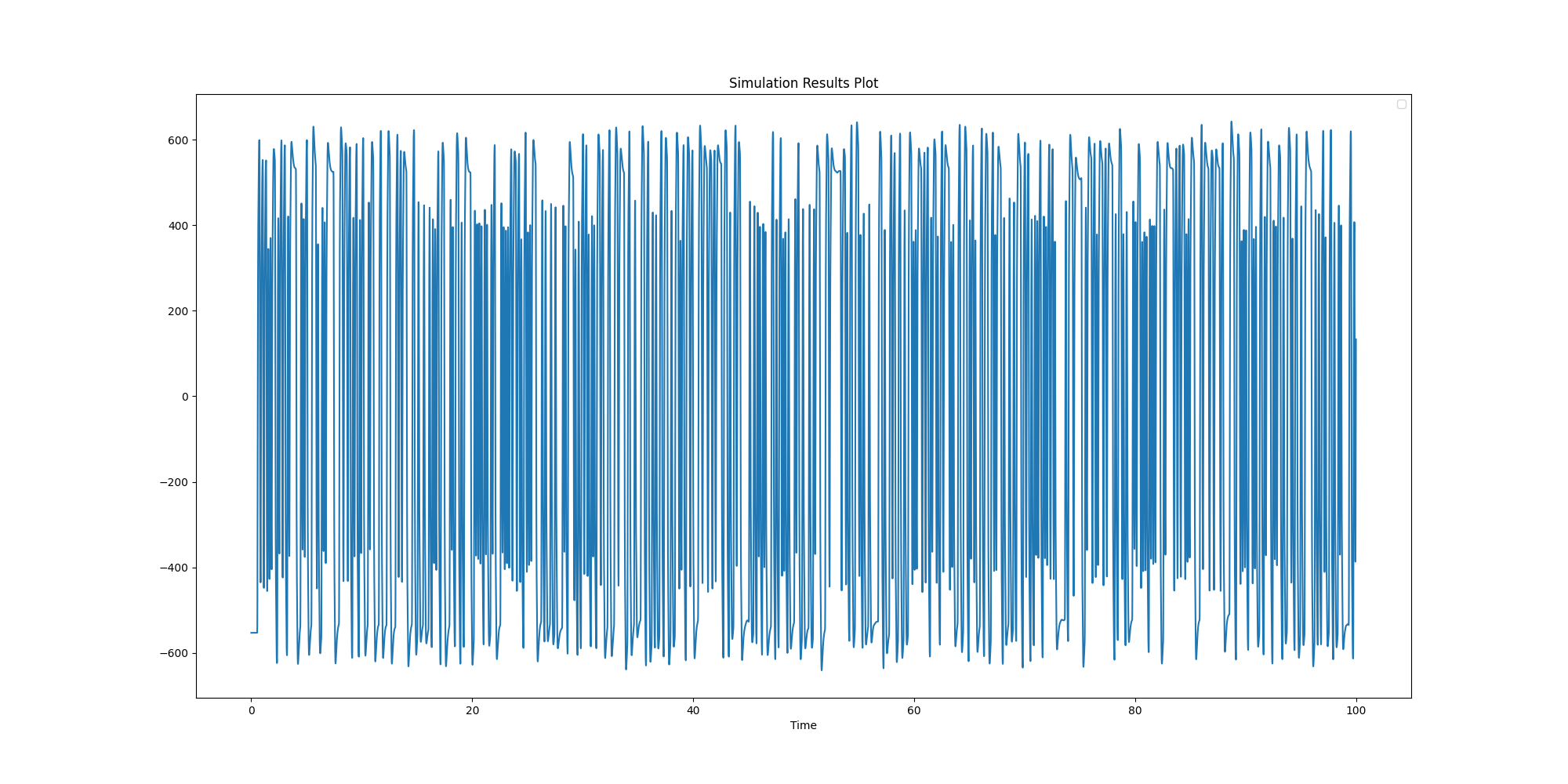
Plot data

Create a plot based on solution data.

fig = original_data.plot()

No artists with labels found to put in legend.  Note that artists whose label start with an underscore are ignored when legend() is called with no argument.

Sample WaveAfterProbe waveform using receiver clock

Extract waveform at specific clock time plus half unit interval

probe_name = "b_input_43"
source_name = "b_output4_42"
plot_type = "WaveAfterProbe"
setup_name = "AMIAnalysis"
ignore_bits = 100
unit_interval = 0.1e-9
sample_waveform = cir.post.sample_ami_waveform(setup=setup_name, probe=probe_name, source=source_name,
                                               variation_list_w_value=cir.available_variations.nominal,
                                               unit_interval=unit_interval, ignore_bits=ignore_bits,
                                               plot_type=plot_type)

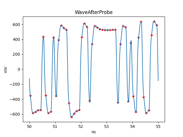
Plot waveform and samples

Create the plot from a start time to stop time in seconds

tstop = 55e-9
tstart = 50e-9
scale_time = pyaedt.constants.unit_converter(1, unit_system="Time", input_units="s",
                                             output_units=original_data.units_sweeps["Time"])
scale_data = pyaedt.constants.unit_converter(1, unit_system="Voltage", input_units="V",
                                             output_units=original_data.units_data[plot_name])

tstop_ns = scale_time * tstop
tstart_ns = scale_time * tstart

for time in original_data_value[plot_name].index:
    if tstart_ns <= time[0]:
        start_index_original_data = time[0]
        break
for time in original_data_value[plot_name][start_index_original_data:].index:
    if time[0] >= tstop_ns:
        stop_index_original_data = time[0]
        break
for time in sample_waveform[0].index:
    if tstart <= time:
        sample_index = sample_waveform[0].index == time
        start_index_waveform = sample_index.tolist().index(True)
        break
for time in sample_waveform[0].index:
    if time >= tstop:
        sample_index = sample_waveform[0].index == time
        stop_index_waveform = sample_index.tolist().index(True)
        break

original_data_zoom = original_data_value[start_index_original_data:stop_index_original_data]
sampled_data_zoom = sample_waveform[0].values[start_index_waveform:stop_index_waveform] * scale_data
sampled_time_zoom = sample_waveform[0].index[start_index_waveform:stop_index_waveform] * scale_time

fig, ax = plt.subplots()
ax.plot(sampled_time_zoom, sampled_data_zoom, "r*")
ax.plot(np.array(list(original_data_zoom.index.values)), original_data_zoom.values)
ax.set_title('WaveAfterProbe')
ax.set_xlabel(original_data.units_sweeps["Time"])
ax.set_ylabel(original_data.units_data[plot_name])
plt.show()

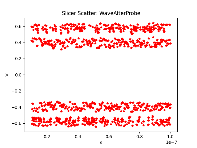
Plot Slicer Scatter

Create the plot from a start time to stop time in seconds

fig, ax2 = plt.subplots()
ax2.plot(sample_waveform[0].index, sample_waveform[0].values, "r*")
ax2.set_title('Slicer Scatter: WaveAfterProbe')
ax2.set_xlabel("s")
ax2.set_ylabel("V")
plt.show()

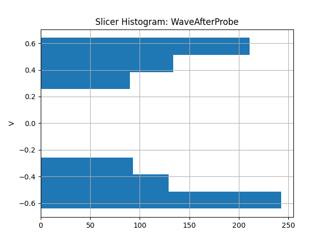
Plot scatter histogram

Create the plot from a start time to stop time in seconds.

fig, ax4 = plt.subplots()
ax4.set_title('Slicer Histogram: WaveAfterProbe')
ax4.hist(sample_waveform[0].values, orientation='horizontal')
ax4.set_ylabel("V")
ax4.grid()
plt.show()

Get Transient report

Get Transient report data

plot_name = "V(b_input_43.int_ami_rx.eye_probe.out)"
cir.solution_type = "NexximTransient"
original_data = cir.post.get_solution_data(expressions=plot_name,
                                           domain="Time",
                                           setup_sweep_name="NexximTransient",
                                           variations=cir.available_variations.nominal)

Sample waveform using a user-defined clock

Extract waveform at specific clock time plus half unit interval.

original_data.enable_pandas_output = False
original_data_value = original_data.data_real()
original_data_sweep = original_data.primary_sweep_values
waveform_unit = original_data.units_data[plot_name]
waveform_sweep_unit = original_data.units_sweeps["Time"]
tics = np.arange(20e-9, 100e-9, 1e-10, dtype=float)

sample_waveform = cir.post.sample_waveform(
    waveform_data=original_data_value,
    waveform_sweep=original_data_sweep,
    waveform_unit=waveform_unit,
    waveform_sweep_unit=waveform_sweep_unit,
    unit_interval=unit_interval,
    clock_tics=tics,
    pandas_enabled=False,
)

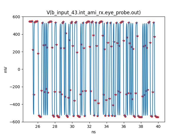
Plot waveform and samples

Create the plot from a start time to stop time in seconds.

tstop = 40.0e-9
tstart = 25.0e-9
scale_time = pyaedt.constants.unit_converter(1, unit_system="Time", input_units="s",
                                             output_units=waveform_sweep_unit)
scale_data = pyaedt.constants.unit_converter(1, unit_system="Voltage", input_units="V",
                                             output_units=waveform_unit)

tstop_ns = scale_time * tstop
tstart_ns = scale_time * tstart

for time in original_data_sweep:
    if tstart_ns <= time:
        start_index_original_data = original_data_sweep.index(time)
        break
for time in original_data_sweep[start_index_original_data:]:
    if time >= tstop_ns:
        stop_index_original_data = original_data_sweep.index(time)
        break
cont = 0
for frame in sample_waveform:
    if tstart <= frame[0]:
        start_index_waveform = cont
        break
    cont += 1
for frame in sample_waveform[start_index_waveform:]:
    if frame[0] >= tstop:
        stop_index_waveform = cont
        break
    cont += 1

original_data_zoom = original_data_value[start_index_original_data:stop_index_original_data]
original_sweep_zoom = original_data_sweep[start_index_original_data:stop_index_original_data]
original_data_zoom_array = np.array(list(map(list, zip(original_sweep_zoom, original_data_zoom))))
original_data_zoom_array[:, 0] *= 1
sampled_data_zoom_array = np.array(sample_waveform[start_index_waveform:stop_index_waveform])
sampled_data_zoom_array[:, 0] *= scale_time
sampled_data_zoom_array[:, 1] *= scale_data

fig, ax = plt.subplots()
ax.plot(sampled_data_zoom_array[:, 0], sampled_data_zoom_array[:, 1], "r*")
ax.plot(original_sweep_zoom, original_data_zoom_array[:, 1])
ax.set_title(plot_name)
ax.set_xlabel(waveform_sweep_unit)
ax.set_ylabel(waveform_unit)
plt.show()

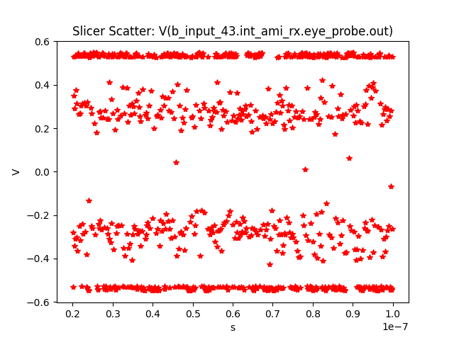
Plot slicer scatter

Create the plot from a start time to stop time in seconds.

sample_waveform_array = np.array(sample_waveform)
fig, ax2 = plt.subplots()
ax2.plot(sample_waveform_array[:, 0], sample_waveform_array[:, 1], "r*")
ax2.set_title('Slicer Scatter: ' + plot_name)
ax2.set_xlabel("s")
ax2.set_ylabel("V")
plt.show()

Save project and close AEDT

Save the project and close AEDT.

cir.save_project()
print("Project Saved in {}".format(cir.project_path))
cir.release_desktop()

Project Saved in D:/Temp/pyaedt_prj_JF6/ami/

True