Advanced#

You can use PyAEDT for postprocessing of AEDT results to display graphics object and plot data.

Touchstone#

TouchstoneData class is based on scikit-rf package and allows advanced touchstone post-processing. The following methods allows to read and check touchstone files.

`TouchstoneData.get_insertion_loss_index`	Get all insertion losses.
`TouchstoneData.plot_insertion_losses`	Plot all insertion losses.
`TouchstoneData.plot`	Plot a list of curves.
`TouchstoneData.plot_return_losses`	Plot all return losses.
`TouchstoneData.get_mixed_mode_touchstone_data`	Transform network from single ended parameters to generalized mixed mode parameters.
`TouchstoneData.get_return_loss_index`	Get the list of all the return loss from a list of excitations.
`TouchstoneData.get_insertion_loss_index_from_prefix`	Get the list of all the insertion losses from prefix.
`TouchstoneData.get_next_xtalk_index`	Get the list of all the Near End XTalk a list of excitation.
`TouchstoneData.get_fext_xtalk_index_from_prefix`	Get the list of all the Far End XTalk from a list of excitations and a prefix that will be used to retrieve driver and receivers names.
`TouchstoneData.plot_next_xtalk_losses`	Plot all next crosstalk curves.
`TouchstoneData.plot_fext_xtalk_losses`	Plot all fext crosstalk curves.
`TouchstoneData.get_worst_curve`	Analyze a solution data object with multiple curves and find the worst curve.
`read_touchstone`	Load the contents of a Touchstone file into an NPort.
`check_touchstone_files`	Check passivity and causality for all Touchstone files included in the folder.
`find_touchstone_files`	Get all Touchstone files in a directory.

Here an example on how to use TouchstoneData class.

from ansys.aedt.core.visualization.advanced.touchstone_parser import TouchstoneData

ts1 = TouchstoneData(touchstone_file=os.path.join(test_T44_dir, "port_order_1234.s8p"))
assert ts1.get_mixed_mode_touchstone_data()
ts2 = TouchstoneData(touchstone_file=os.path.join(test_T44_dir, "port_order_1324.s8p"))
assert ts2.get_mixed_mode_touchstone_data(port_ordering="1324")

assert ts1.plot_insertion_losses(plot=False)
assert ts1.get_worst_curve(curve_list=ts1.get_return_loss_index(), plot=False)

Farfield#

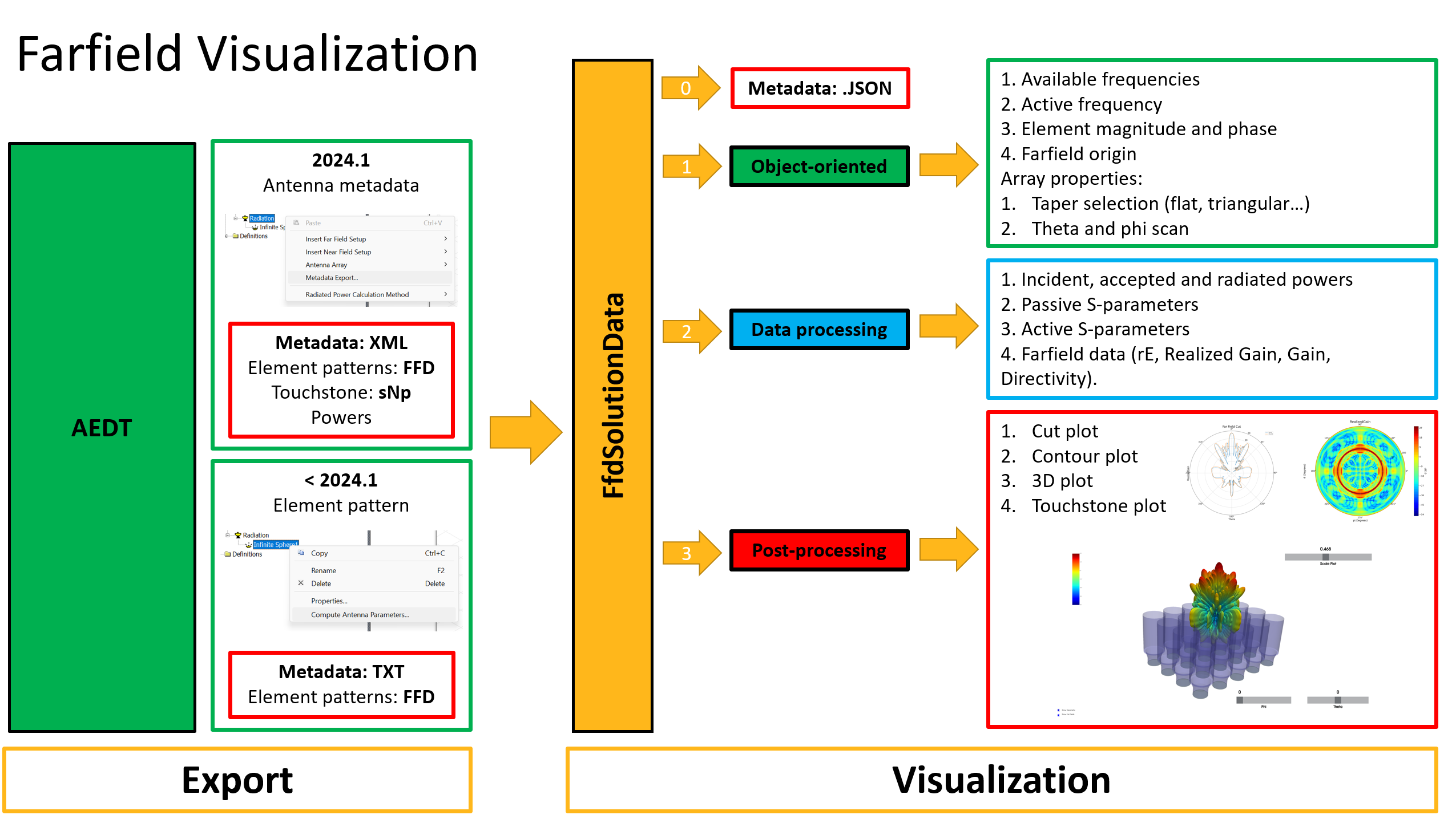
PyAEDT offers sophisticated tools for advanced farfield post-processing. There are two complementary classes: FfdSolutionDataExporter and FfdSolutionData.

FfdSolutionDataExporter: Enables efficient export and manipulation of farfield data. It allows users to convert simulation results into a standard metadata format for further analysis, or reporting.
FfdSolutionData: Focuses on the direct access and processing of farfield solution data. It supports a comprehensive set of postprocessing operations, from visualizing radiation patterns to computing key performance metrics.

FfdSolutionData

Provides antenna far-field data.

This code shows how you can get the farfield data and perform some post-processing:

import ansys.aedt.core
from ansys.aedt.core.generic.farfield_visualization import FfdSolutionDataExporter

app = ansys.aedt.core.Hfss()
ffdata = app.get_antenna_data(
    frequencies=None,
    setup="Setup1 : Sweep",
    sphere="3D",
    variations=None,
    overwrite=False,
    link_to_hfss=True,
    export_touchstone=True,
)
incident_power = ffdata.incident_power
ffdata.plot_cut(primary_sweep="Theta", theta=0)
ffdata.plot_contour(polar=True)
ffdata.plot_3d(show_geometry=False)
app.release_desktop(False, False)

If you exported the farfield data previously, you can directly get the farfield data:

from ansys.aedt.core.generic.farfield_visualization import FfdSolutionData

input_file = r"path_to_ffd\pyaedt_antenna_metadata.json"
ffdata = FfdSolutionData(input_file)
incident_power = ffdata.incident_power
ffdata.plot_cut(primary_sweep="Theta", theta=0)
ffdata.plot_contour(polar=True)
ffdata.plot_3d(show_geometry=False)
app.release_desktop(False, False)

The following diagram shows both classes work. You can use them independently or from the get_antenna_data method.

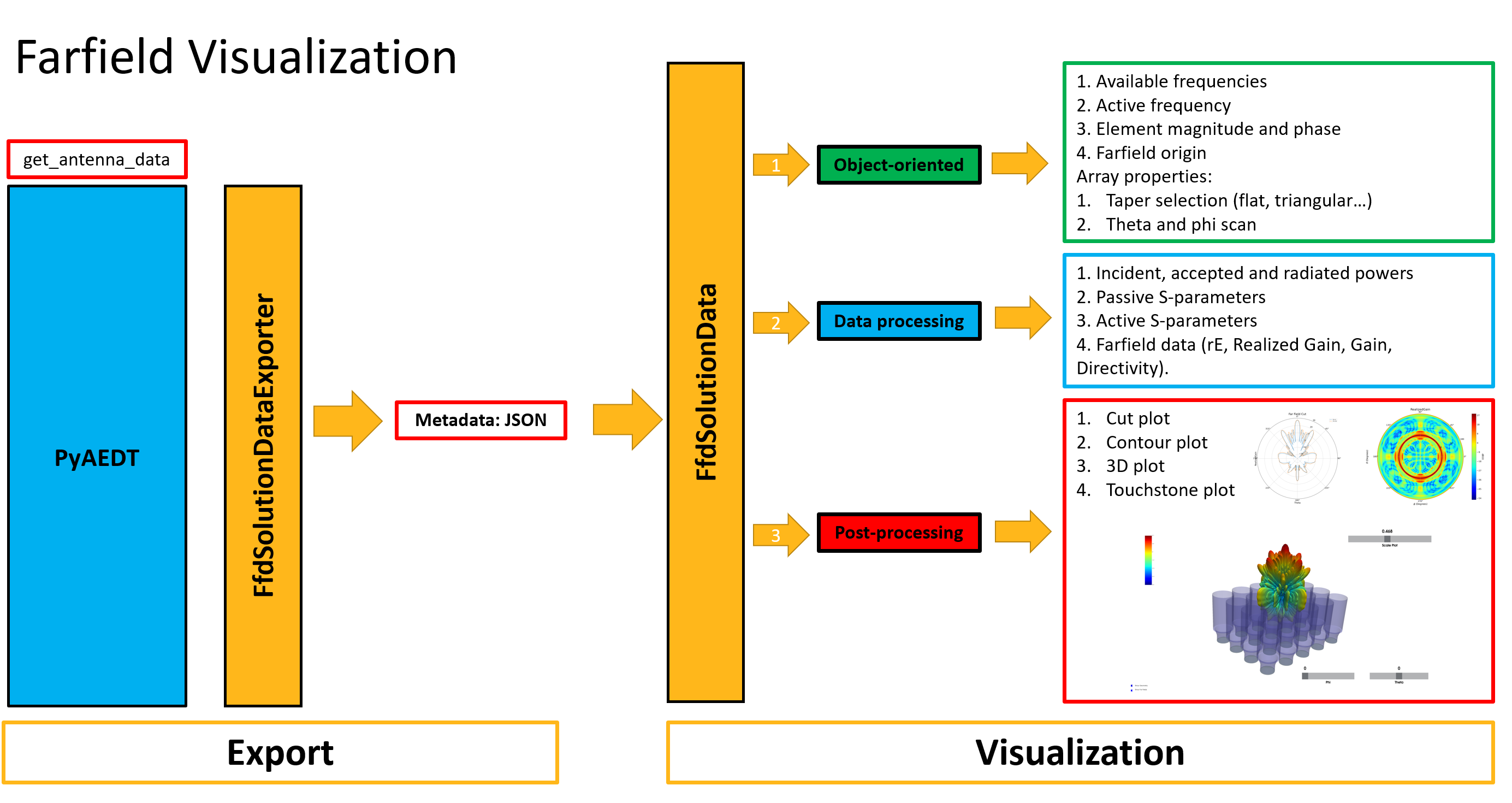
If you have existing farfield data, or you want to export it manually, you can still use FfdSolutionData class.

Monostatic RCS#

PyAEDT provides tools for exporting monostatic radar cross section (RCS) data through the MonostaticRCSExporter class. For advanced RCS post-processing, analysis, and visualization, use the Radar Explorer Toolkit.

Note

Advanced RCS features (MonostaticRCSData and MonostaticRCSPlotter) have been moved to the Radar Explorer Toolkit.

Install the toolkit with:

pip install ansys-aedt-toolkits-radar-explorer

PyAEDT RCS exporter#

The MonostaticRCSExporter class enables efficient export of RCS simulation data into a standardized metadata format for further analysis with the Radar Explorer Toolkit.

MonostaticRCSExporter

Class to enable export of radar cross-section (RCS) data from HFSS.

Export RCS data from HFSS:

from ansys.aedt.core import Hfss

app = Hfss()
setup_name = "Setup1 : LastAdaptive"
frequencies = [77e9]

# Export RCS data
rcs_exporter = app.get_rcs_data(
    frequencies=frequencies, setup=setup_name, variation_name="rcs_solution"
)

# Metadata file is created for use with Radar Explorer Toolkit
metadata_file = rcs_exporter.metadata_file

Radar explorer toolkit#

For comprehensive RCS analysis and visualization, use the radar explorer toolkit:

MonostaticRCSData: Advanced processing of RCS solution data with support for range profiles, waterfall plots, and ISAR imaging.
MonostaticRCSPlotter: Interactive 3D visualization and post-processing of RCS data.

Example using the radar explorer toolkit:

# Install first: pip install ansys-aedt-toolkits-radar-explorer
from ansys.aedt.toolkits.radar_explorer.rcs_visualization import MonostaticRCSData
from ansys.aedt.toolkits.radar_explorer.rcs_visualization import MonostaticRCSPlotter

# Load RCS data exported from PyAEDT
input_file = r"path_to_data\pyaedt_rcs_metadata.json"
rcs_data = MonostaticRCSData(input_file)

# Create plotter for visualization
rcs_plotter = MonostaticRCSPlotter(rcs_data)

# Generate various plots
rcs_plotter.plot_rcs(primary_sweep="IWavePhi")
rcs_plotter.plot_3d()
rcs_plotter.add_range_profile()
rcs_plotter.plot_scene()

For complete documentation and API reference, see:

Radar explorer API

FRTM processing#

PyAEDT offers sophisticated tools for FRTM post-processing. There are two complementary classes: FRTMData, and FRTMPlotter.

FRTMData: Focuses on the direct access and processing of FRTM solution data. It supports a comprehensive set of postprocessing operations, like range profile and range doppler processing.
FRTMPlotter: Focuses on the post-processing of FRTM solution data.

`FRTMData`	Provides FRTM data.
`FRTMPlotter`	Provides range doppler data.

This code shows how you can get the FRTM data:

from ansys.aedt.core.visualization.advanced.frtm_visualization import FRTMPlotter
from ansys.aedt.core.visualization.advanced.frtm_visualization import FRTMData

input_dir = r"path_to_data"

doppler_data_frames = {}
frames_dict = get_results_files(input_dir)

for frame, data_frame in frames_dict.items():
    doppler_data = FRTMData(data_frame)
    doppler_data_frames[frame] = doppler_data

frtm_plotter = FRTMPlotter(doppler_data_frames)
frtm_plotter.plot_range_doppler()

The following picture shows the output of the previous code.

Heterogeneous data message#

Heterogeneous data message (HDM) is the file exported from SBR+ solver containing rays information. The following methods allows to read and plot rays information.

`hdm_plot.HDMPlotter`	Manages Hdm data to be plotted with `pyvista`.
`sbrplus.hdm_parser.Parser`	Parser class that loads an HDM-format export file from HFSS SBR+, interprets its header and its binary content.

Miscellaneous#

PyAEDT has additional advanced post-processing features:

`convert_nearfield_data`	Convert a near field data folder to hfss nfd file and link it to and file.
`parse_rdat_file`	Parse Ansys report '.rdat' file.