Q3D Extractor: busbar analysis

This example shows how you can use PyAEDT to create a busbar design in Q3D Extractor and run a simulation.

Perform required imports

Perform required imports.

import os
import pyaedt

Set non-graphical mode

Set non-graphical mode. You can set non_graphical either to True or False.

non_graphical = False

Set debugger mode

PyAEDT allows to enable a debug logger which logs all methods called and argument passed. This example shows how to enable it.

pyaedt.settings.enable_debug_logger = True
pyaedt.settings.enable_debug_methods_argument_logger = True
pyaedt.settings.enable_debug_internal_methods_logger = False

Launch AEDT and Q3D Extractor

Launch AEDT 2023 R2 in graphical mode and launch Q3D Extractor. This example uses SI units.

q = pyaedt.Q3d(projectname=pyaedt.generate_unique_project_name(),
               specified_version="2023.2",
               non_graphical=non_graphical,
               new_desktop_session=True)

Initializing new desktop!

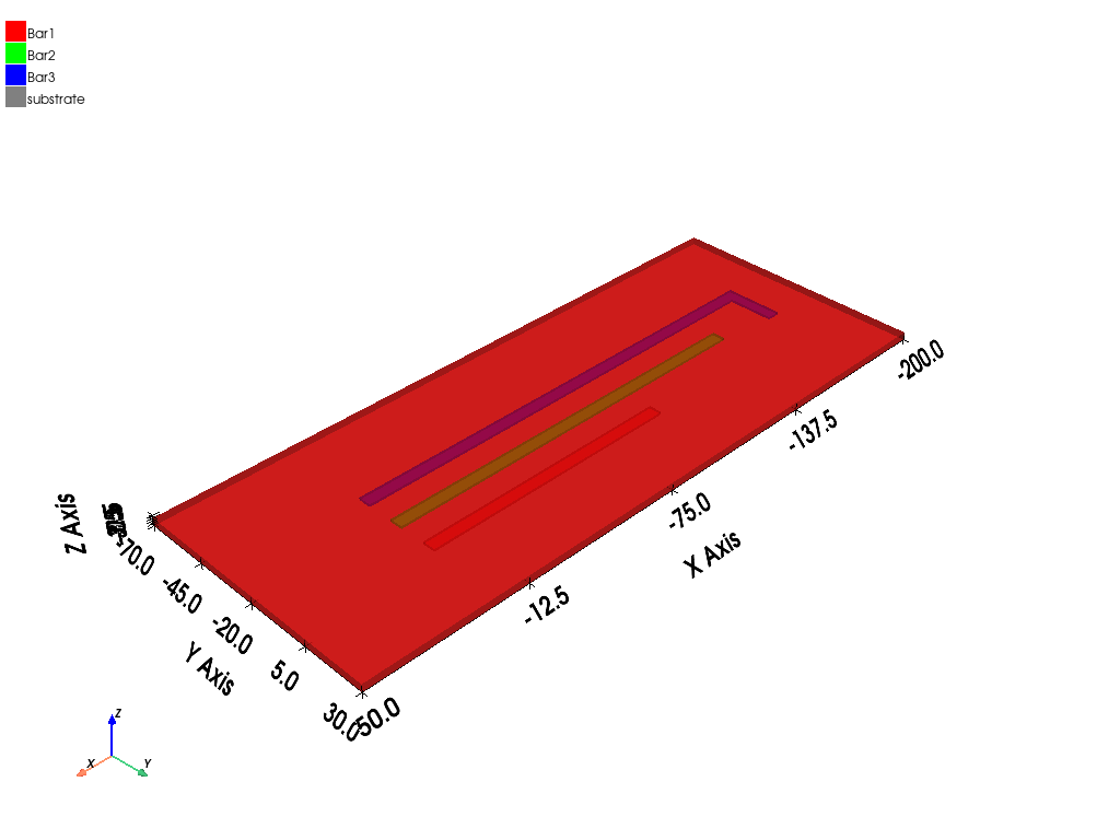
Create primitives

Create polylines for three busbars and a box for the substrate.

b1 = q.modeler.create_polyline(
    [[0, 0, 0], [-100, 0, 0]],
    name="Bar1",
    matname="copper",
    xsection_type="Rectangle",
    xsection_width="5mm",
    xsection_height="1mm",
)
q.modeler["Bar1"].color = (255, 0, 0)

q.modeler.create_polyline(
    [[0, -15, 0], [-150, -15, 0]],
    name="Bar2",
    matname="aluminum",
    xsection_type="Rectangle",
    xsection_width="5mm",
    xsection_height="1mm",
)
q.modeler["Bar2"].color = (0, 255, 0)

q.modeler.create_polyline(
    [[0, -30, 0], [-175, -30, 0], [-175, -10, 0]],
    name="Bar3",
    matname="copper",
    xsection_type="Rectangle",
    xsection_width="5mm",
    xsection_height="1mm",
)
q.modeler["Bar3"].color = (0, 0, 255)

q.modeler.create_box([50, 30, -0.5], [-250, -100, -3], name="substrate", matname="FR4_epoxy")
q.modeler["substrate"].color = (128, 128, 128)
q.modeler["substrate"].transparency = 0.8

q.plot(show=False, export_path=os.path.join(q.working_directory, "Q3D.jpg"), plot_air_objects=False)

<pyaedt.generic.plot.ModelPlotter object at 0x000001D9A4263CD0>

Set up boundaries

Identify nets and assign sources and sinks to all nets. There is a source and sink for each busbar.

q.auto_identify_nets()

q.source("Bar1", axisdir=q.AxisDir.XPos, name="Source1")
q.sink("Bar1", axisdir=q.AxisDir.XNeg, name="Sink1")

q.source("Bar2", axisdir=q.AxisDir.XPos, name="Source2")
q.sink("Bar2", axisdir=q.AxisDir.XNeg, name="Sink2")
q.source("Bar3", axisdir=q.AxisDir.XPos, name="Source3")
bar3_sink = q.sink("Bar3", axisdir=q.AxisDir.YPos)
bar3_sink.name = "Sink3"

Print information

Use the different methods available to print net and terminal information.

print(q.nets)
print(q.net_sinks("Bar1"))
print(q.net_sinks("Bar2"))
print(q.net_sinks("Bar3"))
print(q.net_sources("Bar1"))
print(q.net_sources("Bar2"))
print(q.net_sources("Bar3"))

['Bar1', 'Bar2', 'Bar3']
['Sink1']
['Sink2']
['Sink3']
['Source1']
['Source2']
['Source3']

Create setup

Create a setup for Q3D Extractor and add a sweep that defines the adaptive frequency value.

setup1 = q.create_setup(props={"AdaptiveFreq": "100MHz"})
sw1 = setup1.add_sweep()
sw1.props["RangeStart"] = "1MHz"
sw1.props["RangeEnd"] = "100MHz"
sw1.props["RangeStep"] = "5MHz"
sw1.update()

True

Get curves to plot

Get the curves to plot. The following code simplifies the way to get curves.

data_plot_self = q.matrices[0].get_sources_for_plot(get_self_terms=True, get_mutual_terms=False)
data_plot_mutual = q.get_traces_for_plot(get_self_terms=False, get_mutual_terms=True, category="C")
data_plot_self
data_plot_mutual

['C(Bar1,Bar2)', 'C(Bar1,Bar3)', 'C(Bar2,Bar1)', 'C(Bar2,Bar3)', 'C(Bar3,Bar1)', 'C(Bar3,Bar2)']

Create rectangular plot

Create a rectangular plot and a data table.

q.post.create_report(expressions=data_plot_self)
q.post.create_report(expressions=data_plot_mutual, context="Original", plot_type="Data Table")

<pyaedt.modules.report_templates.Standard object at 0x000001D9A42610F0>

Solve setup

Solve the setup.

q.analyze()
q.save_project()

True

Get report data

Get the report data into a data structure that allows you to manipulate it.

a = q.post.get_solution_data(expressions=data_plot_self, context="Original")
a.intrinsics["Freq"]
a.data_magnitude()
a.plot()

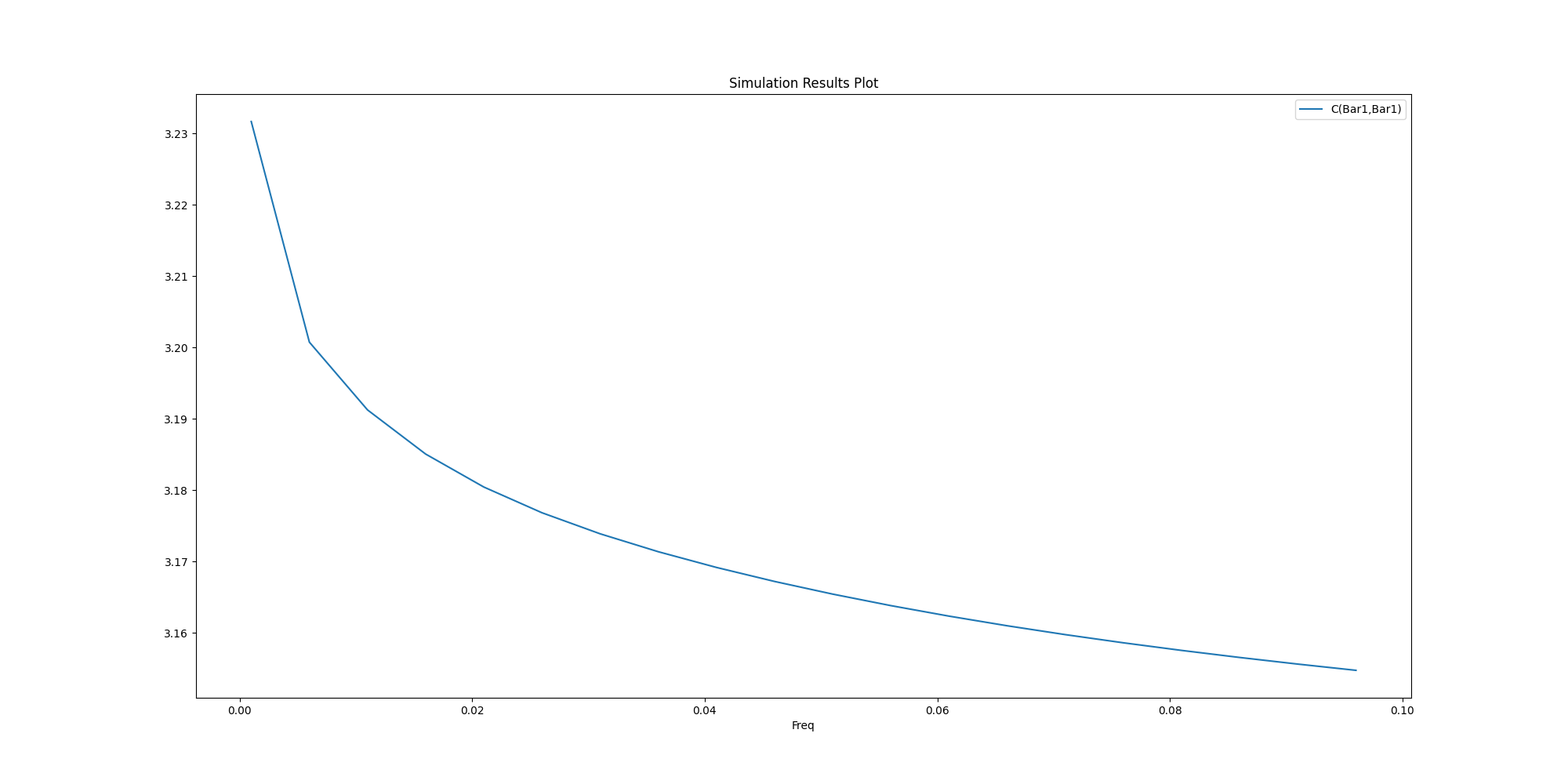
<Figure size 2000x1000 with 1 Axes>

Close AEDT

After the simulation completes, you can close AEDT or release it using the release_desktop method. All methods provide for saving projects before closing.

pyaedt.settings.enable_debug_logger = False
pyaedt.settings.enable_debug_methods_argument_logger = False
q.release_desktop(close_projects=True, close_desktop=True)

True